
Working with NetCDF files in Matlab
NetCDF data files are a great way to share oceanographic data, and they are the primary format supported by the OOI program for data delivery (in addition to .csv and .json). In this tutorial we will walk through a few of Matlab’s basic NetCDF functions that you can use to decode NetCDF files and find out what’s in them. We also recommend checking out NASA’s Panoply software, which provides an easy-to-use freeware tool to investigate the contents of NetCDF files.
First, you’ll need to download a NetCDF datafile to play with. I downloaded the recovered data from deployment #4 of Pioneer Glider 387. You can request the data yourself by going to the Data Portal, and requesting data between 1/1/16 and 1/1/17. The email you receive from the system will point you to a directory that looks like the following…

An example listing of data files provided by the Data Portal when requesting a custom download.
You will want to download the .nc file that contains CTD data. Simply click on the file, and if you are accessing the datafile through the THREDDS server, click on HTTPServer link to download the data file directly to your machine.
Note that when you request glider data, you will often receive GPS data files as part of the response. However, you most likely will not need them, since latitude and longitude data should already be incorporated into the data file. Also, if you are downloading data for use on your local machine, you can ignore .ncml files, which will not work when downloaded. NcML files can provide an easy way to point to aggregated data, when a large data request results in multiple data files, but they only contain internal pointers to other data files, which is why they do not work offline.
Let’s specify a variable which points to the file, so we don’t have to type it out every time.
filename = 'deployment0004_CP05MOAS-GL387-03-CTDGVM000-recovered_host-ctdgv_m_glider_instrument_recovered_20160404T190109.208590-20160714T010519.309690.nc';
Reading File Information
ncinfo() will read all of the metadata contained in the file into a structured array, which you can then peruse in Matlab’s GUI or command line. The following example will load in the metadata, and then display a list of all of the variables contained in the data file.
% Display included Variables
meta = ncinfo(filename);
disp('Variable List');
disp({meta.Variables.Name}');
We can also display a list of the Global Attributes in the file.
% Display Global Attributes
disp('Global Attributes');
disp({meta.Attributes.Name}');
Reading Attributes
The function ncreadatt() can be used to grab a specific attribute’s value.
% Pull the source attribute to use as a plot title
disp('Source Information');
source = ncreadatt(filename,'/','source'); %Get the data stream's name
disp(source);
The source attribute is typically a concatenation of the subsite, node, sensor, collection_method, and stream attributes, which you can also pull individually. The following attributes contain details on the specific instrument used to collect the data: Manufacturer, ModelNumber, SerialNumber, and Description. If you’re interested in the temporal coverage included in the file, you can take a look at time_coverage_start, time_coverage_end (of course, you could also just look at the time variable).
In addition, you can grab the attributes for a specific variable by specifying the variable’s name as the second parameter in ncreadatt(). For example, here’s how to grab the units for the time variable, which was the 2nd variable in the list for me.
disp('Time Variable Attributes');
disp({meta.Variables(2).Attributes.Name}');
disp('Time Units');
disp(ncreadatt(filename,'time','units'))
Load in a Variable
Finally, ncread() can be used to grab the actual data for a specific variable. The following code retrieves time, pressure, temperature, and salinity for this glider.
% Load in a few selected variables
dtime = ncread(filename,'time');
pressure = ncread(filename,'sci_water_pressure_dbar');
temperature = ncread(filename,'sci_water_temp');
temperature(temperature==0)=NaN; %Remove some bad points
salinity = ncread(filename,'practical_salinity');
salinity(salinity==0)=NaN; %Remove some bad points
Note, that the dataset includes date/time as seconds since 1900. (You can confirm this by looking at the units attribute field, as noted above.) The following line converts the time used in the data file to Matlab’s time format so that we can use Matlab’s built-in date/time functions.
dtime = dtime/(60*60*24)+datenum(1900,1,1); %Convert to Matlab time
Now that we have our data, we can plot it up.
% Time Series Plots
figure(1)
subplot(3,1,1)
  plot(dtime,pressure,'.')
  datetick('keeplimits');
  ylabel('Pressure (dbar)')
  title(source,'interpreter','none');
  set(gca,'ydir','reverse'); %Flip the y-axis
subplot(3,1,2)
  plot(dtime,temperature,'.')
  datetick('keeplimits');
  ylabel('Temperature (C)')
subplot(3,1,3)
  plot(dtime,salinity,'.')
  datetick('keeplimits');
  ylabel('Salinity')

print('tutorial1-fig2.png','-dpng');

Time series plots of pressure, temperature and salinity from Pioneer Glider 387, deployed in 2016.
% Profile Plots
figure(2)
subplot(1,2,1)
  plot(temperature,pressure,'.')
  set(gca,'ydir','reverse')
  xlabel('Temperature (C)')
  ylabel('Pressure')
subplot(1,2,2)
  plot(salinity,pressure,'.')
  set(gca,'ydir','reverse')
  xlabel('Salinity')
  t=title(source,'interpreter','none','HorizontalAlignment','right');
  t_pos = get(t,'position');
  xlim = get(gca,'xlim');
  set(t,'position',[xlim(2) t_pos(2)]);

print('tutorial1-fig3.png','-dpng');
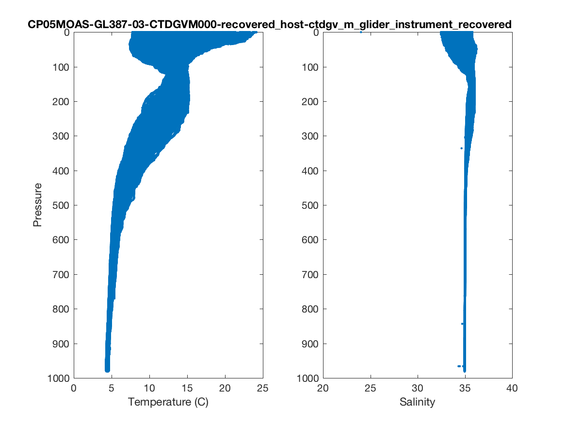
Profile plots of temperature and salinity from Pioneer Glider 387, deployed in 2016.
You’ll notice a few tricks for handling the titles. Setting “interpreter” to none prevents the underscores from converting characters to subscript, which is the default behavior in Matlab. In the second figure, I repositioned the (very long) title to span both subplots.
Well, that’s the quick introduction. Be sure to take a look at the metadata variable to see what else is included in the file, and don’t forget to check out Panoply as well, which makes it very easy to see what’s included in the file. In future tutorials, we’ll demonstrate how to plot this data and others in scientifically useful ways.
— By Sage Lichtenwalner, Last revised on June 28, 2017 —