
THREDDS Quick Start
Contents
How to Browse the THREDDS Data Server
The OOI THREDDS Data Server provides a catalog of pre-generated datasets for some of the most commonly requested instruments that the OOI maintains. You can access this catalog using your favorite OPeNDAP toolboxes, like Pydap for Python or the NetCDF functions in Matlab. The examples shown below can be modified for OOI’s “Gold-Copy” THREDDS server.
THREDDS ServerDatasets in the catalog are structured in the following way:
The Site-Platform Code is an 8 character code the specifies a particular mooring, seafloor node or collection of mobile assets. To translate these codes, please check out the list of Site-Platform Codes.
The Instrument Code is a 12 character code, but the most useful part is the 5 digets following the dash which specifies the Instrument Class (e.g. CTDPF=CTD Profiler, FLORT=3-Wavelength Flourormeter, etc.). To translate these codes, please check out the list of Instrument Class Codes.
For example, if you were interested in recovered CTD data from a glider at the Pioneer Array, you would navigate to:
Coastal_Pioneer/CP05MOAS/03-CTDGVM000/recovered_host
At this point, you will see a list of data streams, In this case each data stream is for an individual glider at the Array.
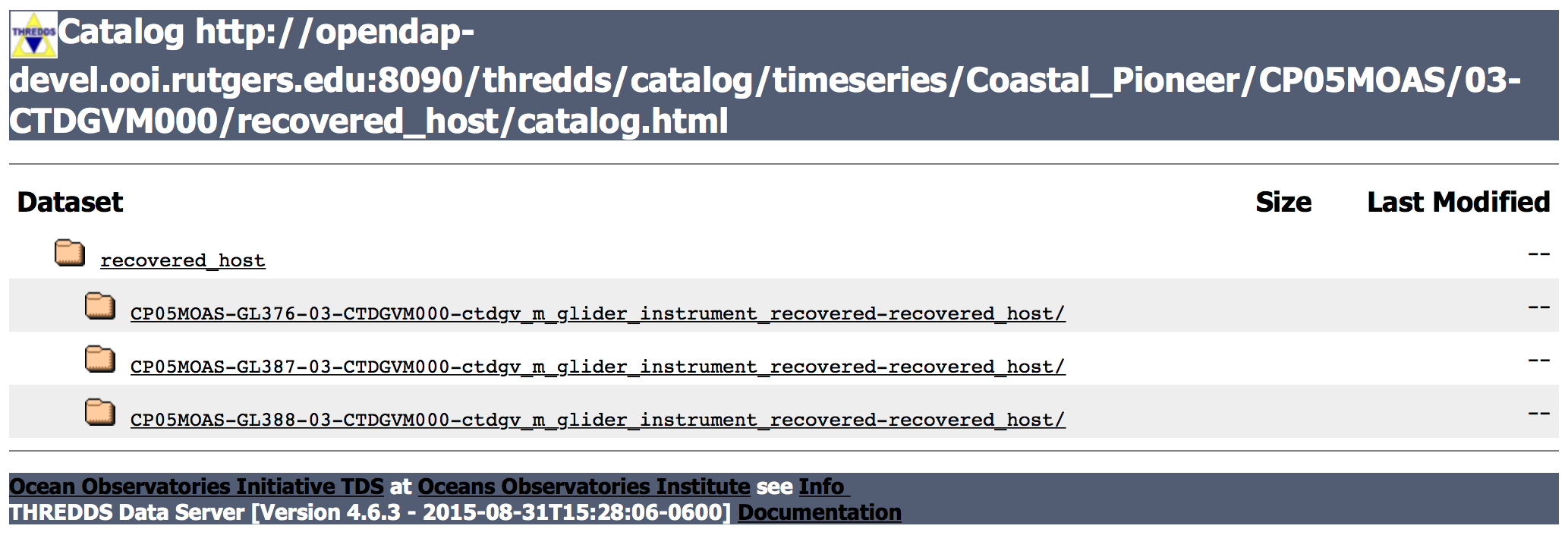
THREDDS Catalog image showing the CTD datasets from CP05MOAS
Choosing a particular stream will then take you to the dataset list for that particular data stream.
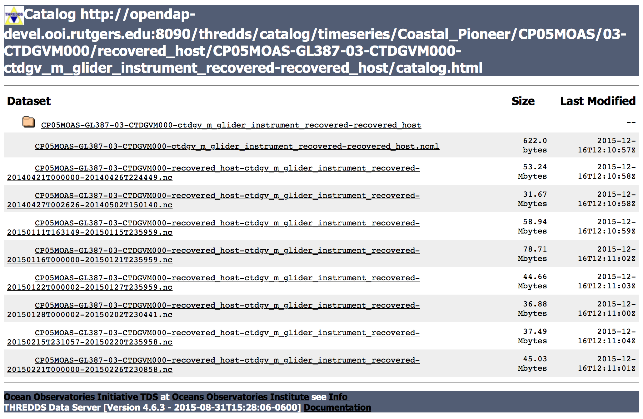
THREDDS catalog screenshot showing the CTD datasets for Glider 387 at the Pioneer Array.
This page lists two kinds of files which provide different capabilities. You can choose the best one depending on your need.
1) The fist entry on this page is a .ncml file, which is an aggregated dataset. If you are using an OPeNDAP connector, this is the dataset you will want to use as it contains data for all possible times that are available. Click on this file, and then choose the “OPENDAP” url presented on the page to use in your program. (See below for an example Matlab script.)
2) The other entries on the page are individual datasets that include data only for specific time periods. While you can also connect to these datasets via an OPeNDAP connector, the advantage of these files is that you can also immediately download them as NetCDF files for offline processing. Click on the file you are interested in, and then on the next page, click on the “HTTPServer” link to download the file.
You can use NASA’s Panoply software to quickly investigate the contents of netCDF files. With the tool, you can quickly browse the variables, variable attributes, and other metadata included in the file. It allows you to create some quick plots of the data.
Example Matlab Script
The following script shows how you can access data on the OOI THREDDS Data Server using the NetCDF functions in Matlab.
First, let’s specify a .ncml URL for the dataset we want to access. In this example, we will grabbing CTD data from Glider 387 deployed at the Pioneer Array.
url='http://opendap-devel.ooi.rutgers.edu:8090/thredds/dodsC/timeseries/Coastal_Pioneer/CP05MOAS/03-CTDGVM000/recovered_host/CP05MOAS-GL387-03-CTDGVM000-ctdgv_m_glider_instrument_recovered-recovered_host/CP05MOAS-GL387-03-CTDGVM000-ctdgv_m_glider_instrument_recovered-recovered_host.ncml';
You can use ncinfo() to access the list of variables and metadata information contained in the dataset.
% Display included Variables
meta = ncinfo(url);
disp({meta.Variables.Name}');
The function ncreadatt() can be used to grab a specific attribute value.
% Pull the source attribute to use as a plot title
source = ncreadatt(url,'/','source'); %Get the data stream name
And ncread() can be used to grab actual data for specific variables. The following code retrieves time, pressure, temperature, and salinity for this glider. Note that the dataset includes date/time data as seconds from 1900. (You can confirm this using ncreadatt(url,’time’,’units’)). The following script converts the time used in the file to Matlab’s time format so that Matlab’s built-in date/time functions can be used.
% Load in a few selected variables
dtime = ncread(url,'time');
dtime = dtime/(60*60*24)+datenum(1900,1,1); %Convert to Matlab time
pressure = ncread(url,'sci_water_pressure');
temperature = ncread(url,'sci_water_temp');
temperature(temperature==0)=NaN; %Remove some bad points
salinity = ncread(url,'sci_water_pracsal');
salinity(salinity==0)=NaN; %Remove some bad points
Now that we have our data, we can make some pretty plots.
% Time Series Plots
figure(1)
subplot(2,2,1)
  plot(dtime,temperature,'.')
  datetick('keeplimits');
  ylabel('Temperature (C)')
subplot(2,2,3)
  plot(dtime,salinity,'.')
  datetick('keeplimits');
  ylabel('Salinity')
subplot(1,4,3)
  plot(temperature,pressure,'.')
  set(gca,'ydir','reverse')
  xlabel('Temperature (C)')
  ylabel('Pressure')
subplot(1,4,4)
  plot(salinity,pressure,'.')
  set(gca,'ydir','reverse')
  xlabel('Salinity')
  t=title(source,'interpreter','none','HorizontalAlignment','right');
  t_pos = get(t,'position');
  xlim = get(gca,'xlim');
  set(t,'position',[xlim(2) t_pos(2)]);

print('fig1.png','-dpng');

% Colored Scatterplots
figure(2)
subplot(2,1,1)
  scatter3(dtime,pressure,0*dtime,32,temperature,'.');
  view([0 -90]);
  datetick('keeplimits');
  ylabel('Pressure')
  cbh=colorbar;
  ylabel(cbh,'Temperature (C)');
  title(source,'interpreter','none')
subplot(2,1,2)
  scatter3(dtime,pressure,0*dtime,32,salinity,'.');
  view([0 -90]);
  datetick('keeplimits');
  ylabel('Pressure')
  cbh=colorbar;
  ylabel(cbh,'Salinity');
  xlabel([datestr(dtime(1),'mmm dd, yyyy') ' to ' datestr(dtime(end),'mmm dd, yyyy')]);

print('fig2.png','-dpng');
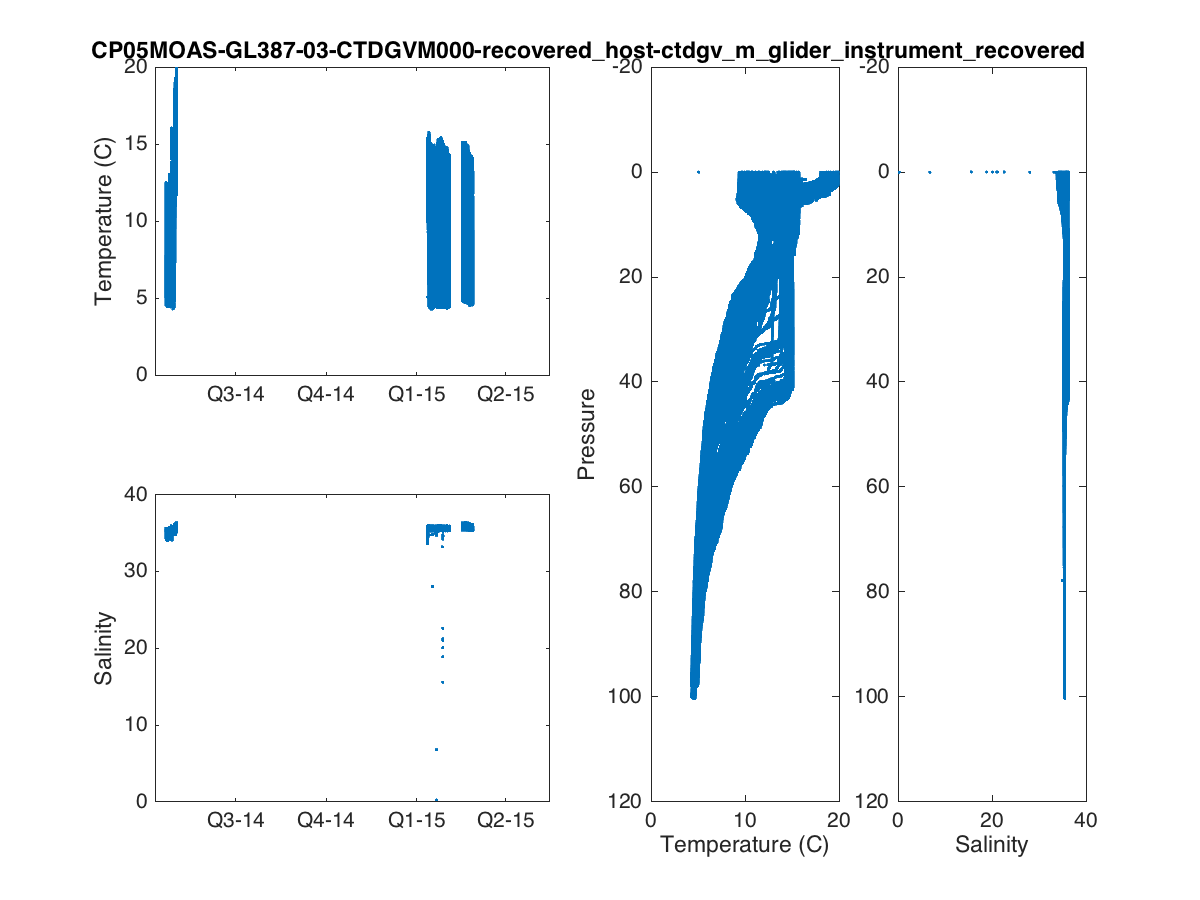
Example Matlab plot showing timeseries of temperature and salinity, and corresponding TS diagram.
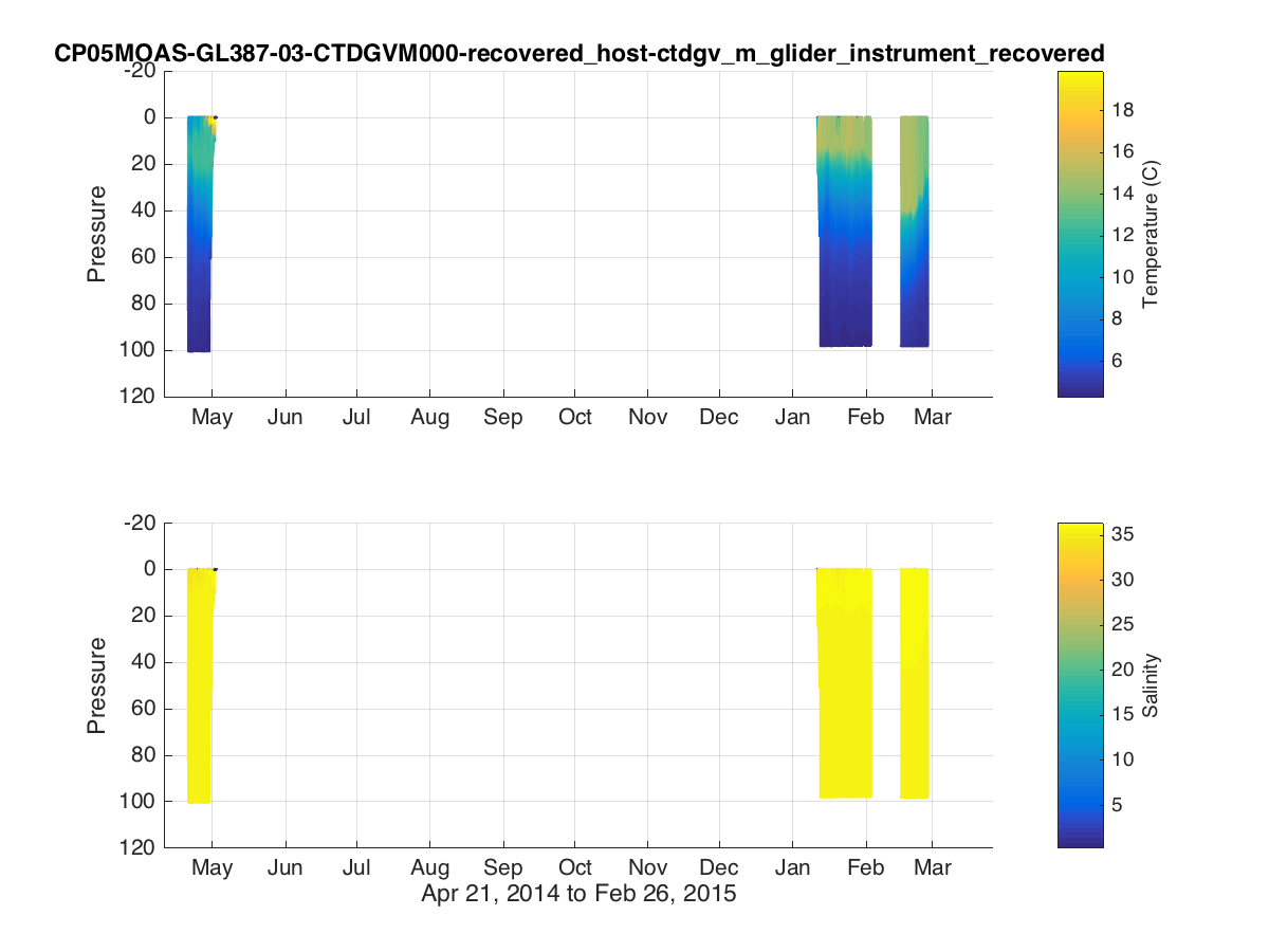
Example Matlab plot showing a colored timeseries glider transect of temperature and salinity.
Note, the example above grabs data for the full range of time in the dataset. If you only want a subset of the full dataset, you can add additional parameters to the ncread() function.
% Instead of extracting the full array, we can select a specific subset
ind = find(dtime>datenum(2015,1,15) & dtime<datenum(2015,1,20));
dtime2 = ncread(url,'time',ind(1),length(ind),1);
dtime2 = dtime2/(60*60*24)+datenum(1900,1,1); %Convert to Matlab time
pressure2 = ncread(url,'sci_water_pressure',ind(1),length(ind),1);
temperature2 = ncread(url,'sci_water_temp',ind(1),length(ind),1);
temperature2(temperature2==0)=NaN; %Remove some bad points
salinity2 = ncread(url,'sci_water_pracsal',ind(1),length(ind),1);
salinity2(salinity2==0)=NaN; %Remove some bad points
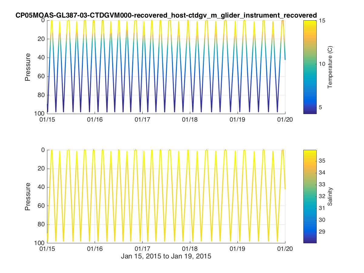
Example Matlab plot showing a colored timeseries glider transect of temperature and salinity for a subsetted dataset.
Hopefully this gives you a quick start on how to grab some basic datasets from the OOI THREDDS Data Server using Matlab. You can find more information in Matlab’s documentation for ncinfo(), ncreadatt(), and ncread().
Example Python Script
The following script shows how you can access data on the OOI THREDDS Data Server using the Pydap library in Python.
Next we specify the dataset we want to use and open the Pydap connection. In this example, we will grab CTD data from Glider 387 deployed at the Pioneer Array, using the aggregrated dataset that ends in .ncml.
First, we need to import the open_url() function from the Pydap library.
from pydap.client import open_url
Next we specify the dataset we want to use and open the Pydap connection. In this example, we will grab CTD data from Glider 387 deployed at the Pioneer Array, using the aggregrated dataset that ends in .ncml.
url = 'http://opendap-devel.ooi.rutgers.edu:8090/thredds/dodsC/timeseries/Coastal_Pioneer/CP05MOAS/03-CTDGVM000/recovered_host/CP05MOAS-GL387-03-CTDGVM000-ctdgv_m_glider_instrument_recovered-recovered_host/CP05MOAS-GL387-03-CTDGVM000-ctdgv_m_glider_instrument_recovered-recovered_host.ncml';
dataset=open_url(url)
You can use the .keys() function to find out which variables are in the dataset.
print dataset.keys()
You can use the following commands to learn more about specific variables in the dataset
dataset['sci_water_temp'].dimensions
dataset['sci_water_temp'].shape
dataset['sci_water_temp'].type
dataset['sci_water_temp'].attributes
Now let’s grab some data for a few different variables. Using [:] will grab all available data in the file. You may want to subset your query if the dataset is rather large.
time = dataset['time'][:]
pressure = dataset['sci_water_pressure'][:]
temp = dataset['sci_water_temp'][:]
sal = dataset['sci_water_pracsal'][:]
Next need to convert the time variable. The dataset includes date/time data as seconds from 1900. (You can confirm this with dataset[‘time’].units) The following line converts the time used in the file so that Matplotlib’s built-in date/time functions can be used.
from datetime import datetime
dtime = time/(24*3600) + datetime(1900,1,1).toordinal()
Now let’s make a plot.
#Import necessary libraries
import numpy as np
import matplotlib.pyplot as plt
import matplotlib.dates as mdates

# Close any existing plots
plt.close('all')

# Setup the plot
fig, ax = plt.subplots()

# Turn on the plot grid
plt.grid()

# Add the scatterplot with data
sc = plt.scatter(dtime,pressure, c=np.abs(temp), marker='o', edgecolor='none')

# Format the date axis
df = mdates.DateFormatter('%Y-%m-%d')
ax.xaxis.set_major_formatter(df)
fig.autofmt_xdate()

# Reverse the y-axis
ax.set_ylim(ax.get_ylim()[::-1])

# Plot lables
plt.ylabel(dataset['sci_water_pressure'].name+" ("+ dataset['sci_water_pressure'].units + ")")
plt.title(dataset.attributes['NC_GLOBAL']['source'], fontsize=11)

# Add the colorbar
clabel = dataset['sci_water_temp'].name +" ("+ dataset['sci_water_temp'].units + ")"
fig.colorbar(sc, ax=ax, label=clabel)

# Display the plot (this is a necessary step in Python) and save the figure to a file.
plt.show()
fig.savefig('pydap_fig1.png')
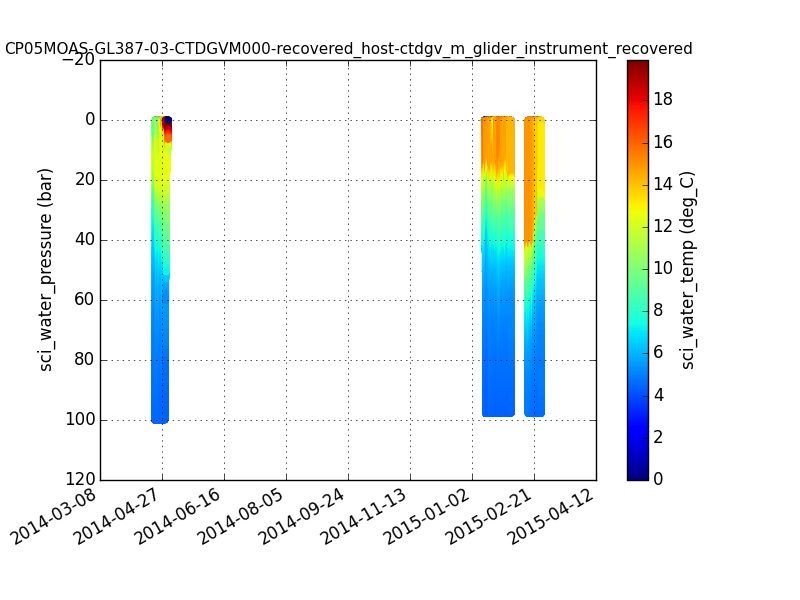
Example Matplotlib plot created in Python showing a colored timeseries glider transect of temperature.
Hopefully this gives you a quick start on how to grab some basic datasets from the OOI THREDDS Data Server using Python. You can find more information in the Pydap documentation.