Making a Glider Deployment Map in Matlab
While most OOI datasets are from fixed assets, like moorings and seafloor nodes, the observatory also includes data from several dozen gliders which move around the arrays. In this tutorial, we will demonstrate how to plot their tracks using data downloaded from the Data Portal, and we will also introduce how to access and plot high-resolution bathymetry from Grid Server.
We’re going to use the same data file as the Working with NetCDF files in Matlab tutorial, so if you want to follow along, take a look at that tutorial for more information on how to obtain and open the file.
Plotting the Track Data
First, we’ll specify a variable which points to the file we have already downloaded, so we don’t have to type it out every time, and then we’ll load in the latitude and longitude track data.
% Data file
filename = 'deployment0004_CP05MOAS-GL387-03-CTDGVM000-recovered_host-ctdgv_m_glider_instrument_recovered_20160404T190109.208590-20160714T010519.309690.nc';

% Load in tie and convert to Matlab time
dtime = ncread(filename,'time');
dtime = dtime/(60*60*24)+datenum(1900,1,1);

% Load in a few selected variables
latitude = ncread(filename,'lat');
longitude = ncread(filename,'lon');
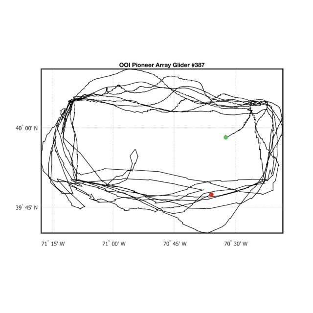
Let’s go ahead and create a simple track map. We’ll use Matlab’s Mapping Toolbox, because it can easily handle different projections if needed, and it also includes a number of functions that make plotting spatial data easier.
% Setup the Map Axes
axesm('MapProjection','mercator');
minlat=min(latitude); maxlat=max(latitude);
minlon=min(longitude); maxlon=max(longitude);
setm(gca, 'MapLatLimit',[minlat maxlat],'MapLonLimit',[minlon maxlon])
setm(gca,'FontWeight','normal','FontSize',10,'FontName','Tahoma','LabelUnits','dm');

% Add lat/lon tickmarks for every degree if the map spans
% greater than 1.5 degrees longitude, or every quarter degree if less.
if abs(maxlon-minlon)>1.5
  setm(gca,'MLineLocation',1,'MLabelLocation',1,'MeridianLabel','on','MLabelParallel','south');
  setm(gca,'PLineLocation',1,'PLabelLocation',1,'ParallelLabel','on','PLabelMeridian','west');
else
  setm(gca,'MLineLocation',0.25,'MLabelLocation',0.25,'MeridianLabel','on','MLabelParallel','south');
  setm(gca,'PLineLocation',0.25,'PLabelLocation',0.25,'ParallelLabel','on','PLabelMeridian','west');
end

% Specify some colors
green = [102,189,99]/255;
red = [215,48,39]/255;

% Plot the Trajectory
p1 = plotm(latitude,longitude,'k-','linewidth',1); %Full Track
hold on;
p2 = plotm(latitude(1),longitude(1),'.','markersize',28,'color',green); %Starting Point
p3 = plotm(latitude(end),longitude(end),'.','markersize',28,'color',red); %Ending Point

% Add a figure title
fig_title = 'OOI Pioneer Array Glider #387';
title(fig_title);

% Additional tweaks to improve the map
tightmap; %Tighten up the map area shown
framem on; %Turn on the black frame
gridm on; %Turn on grid lines

% Save the figure
set(gcf,'PaperPosition',[0.25 0.5 8 8]);
print(gcf,'-dpng','-r300', 'tutorial3-fig1');

Figure 1. A map of the track flown by Pioneer Glider 387 during its 4th deployment in 2016. The start and ending points are shown by the green/red dots respectively.
Adding the Pioneer Moorings
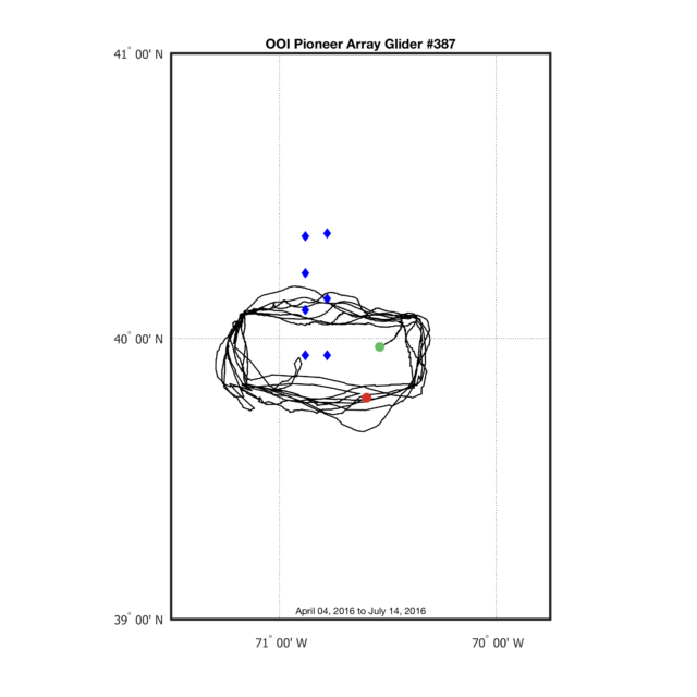
Now we have a simple map of the glider track, but let’s try to put this data into some context. First, let’s expand the map to cover the entire Pioneer Array region.
% Pioneer Lat/Lon Limits
ll = [-71.5 39; -69.75 41];
setm(gca, 'MapLatLimit',[ll(1,2) ll(2,2)],...
          'MapLonLimit',[ll(1,1) ll(2,1)]);
setm(gca,'MLineLocation',1,'MLabelLocation',1,...
    'MeridianLabel','on','MLabelParallel','south');
setm(gca,'PLineLocation',1,'PLabelLocation',1,...
    'ParallelLabel','on','PLabelMeridian','west');
tightmap;
Next, let’s add the rough locations of Pioneer Moorings, which we can get from the individual Site/Platform pages for each mooring in the Pioneer Array.
% Pioneer Moorings (rough locations)
moorings = [-70.78 40.14 %CNSP
  -70.88 40.23 %CP02PMCI
  -70.88 40.10 %CP02PMCO
  -70.78 40.37 %CP02PMUI
  -70.78 39.94 %CP02PMUO
  -70.88 40.36 %CP03ISSP
  -70.88 39.94 %CP04OSPM
];
pm = plotm(moorings(:,2),moorings(:,1),'bd','MarkerFaceColor','b');
Finally, let’s add an annotation that shows the date range of the glider track data, and then we’ll save the new version.
% Date Range Annotation
a1 = textm(39.03,-70.6250,[datestr(dtime(1),'mmmm dd, yyyy') ' to ' datestr(dtime(end),'mmmm dd, yyyy')],'fontsize',8,'HorizontalAlignment','center','color','k');

% Save the figure
print(gcf,'-dpng','-r300', 'tutorial3-fig2');
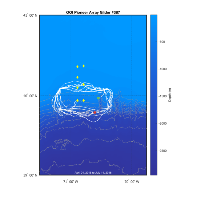
Adding Bathymetry from MGDS
Once we have the glider track plotted, we can improve the map by adding some bathymetry. Above, we specified the lat and lon limits of the full Pioneer Array. If we didn’t already know the range of the data we wanted to show, we could use the next two lines to give us the Latitude and Longitude limits of the dataset.
disp(sprintf('Latitude Range: %g, %g',min(latitude),max(latitude)));
disp(sprintf('Longitude Range: %g, %g',min(longitude),max(longitude)));
After we have the limits we want, we can use them to grab high-resolution bathymetry from MGDS’s Web Services. To do so, simply tweak the following URL with the lat/lon limits you want to download a Global Multi-Resolution Topography (GMRT) data file.
The easiest way to load this datafile into Matlab is with the function grdread2(), available in the Matlab File Exchange.
% Add grdread2 to the path
addpath grdread2

% Specify the bathymetry filename
grd = 'GMRTv3_2_20161202topo_pioneer.grd';

% Load in the bathymetry data
[mx,my,mz]=grdread2(grd);
mz=double(mz);

% Add colored bathymetry
pb = surfm(my,mx,mz);
uistack(pb,'bottom'); % Move the bathy data to the bottom of the figure

% Bathymetry contour lines, every 250m
[cc,pc] = contourm(my,mx,mz,[-3000:250:0],'LineColor',0.6*[1 1 1]);

% Add a colorbar
cbh = colorbar('vert');
ylabel(cbh,'Depth (m)');
Next, we’re going to use a custom colormap for the bathymetry, based on Matplotlib’s terrain colormap.
% Custom colormap for bathymetry
terrain_sea = [
  0.2, 0.2, 0.6;
  0.0, 0.6, 1.0];

terrain_land = [
  0.0, 0.8, 0.4;
  1.0, 1.0, 0.6;
  0.5, 0.36, 0.33;
  1.0, 1.0, 1.0];

demcmap(mz,64,terrain_sea,terrain_land);
Finally, we need to tweak the colors of the plots we added before, so they look nice on the new bathymetry we’re adding to the background.
% Change some plot colors to work on the bathymetry
set(p1,'color','w');
set(pm,'color','y','MarkerFaceColor','y');
set(a1,'color','w');

% Save the figure
print(gcf,'-dpng','-r300', 'tutorial3-fig3');
One more view
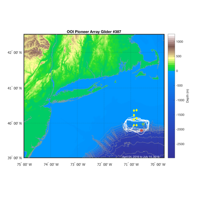
The code above produces a nice map of the glider track on top of some high-resolution bathymetry. However, to add some more context, let’s zoom out a bit to show the Mid-Atlantic coastline as well, so we can really see where the Pioneer Array is. We’ll need to download a new data file from MGDS, which will now include both bathymetry and topography, since the expanded region includes land as well.
% Remove the previous bathymetry plot
delete([pb,pc])

% New Lat/Lon Limits
ll = [-75 39; -69.75 42.5];
setm(gca, 'MapLatLimit',[ll(1,2) ll(2,2)],...
          'MapLonLimit',[ll(1,1) ll(2,1)]);
setm(gca,'MLineLocation',1,'MLabelLocation',1,...
    'MeridianLabel','on','MLabelParallel','south');
setm(gca,'PLineLocation',1,'PLabelLocation',1,...
    'ParallelLabel','on','PLabelMeridian','west');
tightmap;

% Specify the new bathymetry filename
grd = 'GMRTv3_3_20170630topo.grd';

% Load in the bathymetry data
[mx,my,mz]=grdread2(grd);
mz=double(mz);

% Add colored bathymetry
pb = surfm(my,mx,mz);
uistack(pb,'bottom'); % Move the bathy data to the bottom of the figure

% Bathymetry contour lines, every 250m
[cc,pc] = contourm(my,mx,mz,[-3000:250:0],'LineColor',0.6*[1 1 1]);

% Recalculate the colomap
demcmap(mz,64,terrain_sea,terrain_land);

% Save the figure
print(gcf,'-dpng','-r300', 'tutorial3-fig4');

Figure 4. A map showing a portion of the Mid-Atlantic Bight, including the Pioneer Array moorings and the track flown by Pioneer Glider 387 during its 4th deployment in 2016.
And there we have it. Now we can see where the Pioneer Array is in relation to the Mid-Atlantic coast as well as the track of the glider.
Perhaps more importantly, we can also see that this particular glider was flying the Frontal Zone (FZ) sampling pattern, as defined in the Pioneer Array Mobile Asset sampling plan. For more information on the glider sampling patterns at all of the OOI Arrays, please check out the Observation and Sampling Approach page.
— By Sage Lichtenwalner, Last revised on June 29, 2017 —


