
Science Highlights
Shelfbreak Jet Influence on Coastal Sea Level
Flooding and shoreline erosion are increasing threats to coastal communities. Coastal sea levels are influenced by multiple factors, including mean sea level rise, tides, storm surges, river outflow, and waves. A recent paper by Camargo et al. (2025) focused on the extent to which offshore circulation, in particular the shelfbreak jet on the New England shelf, contributed to sea level variability over the period 2014 – 2022. They found that roughly 30% of sea level variance during storm surges can be attributed to the shelfbreak jet.
The authors used a variety of data sets, including tide gauge stations along the New England coastline from Boston, MA to Atlantic City, NJ, wind stress from the ECMWF ERA-5 reanalysis, and shelfbreak jet transport from the OOI Pioneer Array. The jet transport was estimated using upward-looking ADCP data from the Central Inshore, Central, and Central Offshore moorings. The methodology and results are described in Carmargo et al., 2024 and the jet transport data set is available in Zenodo (Carmago, 2024). The data were de-tided and then band-pass filtered (1-15 days) to isolate the storm-surge component of sea level variability. Coherence between coastal sea level and jet transport for 1-15 day periods was established by Carmago et al. (2024).
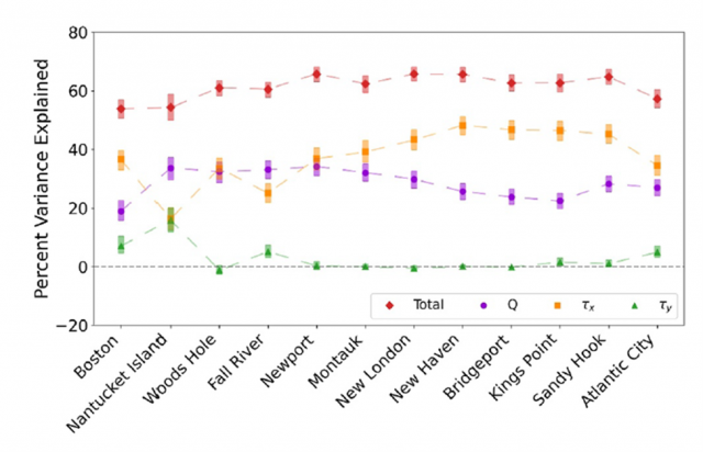
[caption id="attachment_37571" align="alignnone" width="975"]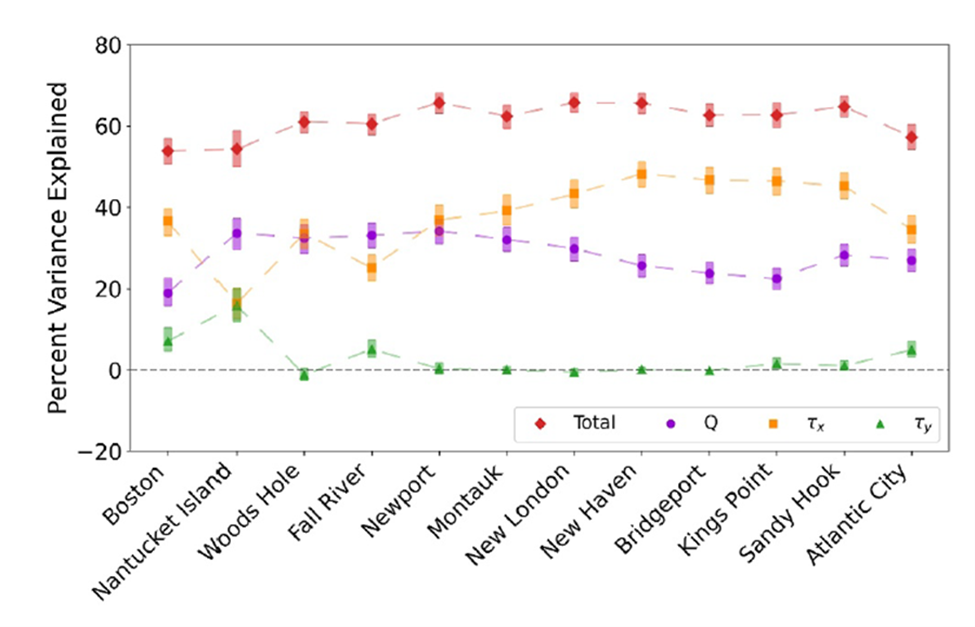 Percent of storm surge variance explained by the regression model (red) and for individual parameters: shelfbreak jet (purple), zonal wind stress (orange), and meridional wind stress (green). Tide gauge stations are ordered from north to south along the coastline. From Camargo et al., 2025.[/caption]
The influence of jet transport and two components of wind stress (zonal and meridional) on storm surge was evaluated by means of a linear regression model that determined the regression coefficients for each parameter. The regression was run for each tide station using the previously computed jet transport and the ERA-5 wind stress closest to each station. Overall, the regression model explained about 60% of the storm surge variance, with jet transport and zonal wind stress explaining 28% and 38%, respectively. There was modest along-coast variability in the variance explained by each parameter (Figure 3): Variance explained by zonal wind stress tended to increase from NE to SW along the coast (Fall River to Bridgeport), while variance explained by the jet tended to decrease. The wind stress impact was identified as due to either onshore or downwelling-favorable winds. The jet impact was due to changes in the cross-shelf pressure gradient associated with the geostrophically-balanced currentCase studies for specific synoptic events highlight the complexity of coastal storm surge events and the broad suite of observational tools necessary to determine the influence of different mechanisms. The authors note that simple storm surge models will not capture the influence of offshore currents like the shelfbreak jet, and that such influence is likely to be found elsewhere on the US east and west coast.
___________________
References:
Camargo, C.M.L., C.G. Piecuch and B. Raubenheimer, 2025. Do ocean dynamics contribute to coastal floods? A case study of the shelfbreak jet and coastal sea level along southern New England, Earth’s Future, 13, https://doi.org/10.1029/2025EF006708.
Camargo, C. M. L. (2024). Shelfbreak jet transport from OOI pioneer [Dataset]. https://doi.org/10.5281/zenodo.10814048.
Camargo, C. M. L., Piecuch, C. G., & Raubenheimer, B. (2024). From shelfbreak to shoreline: Coastal sea level and local ocean dynamics in the Northwest Atlantic. Geophysical Research Letters, 51(14), e2024GL109583. https://doi.org/10.1029/2024GL109583 .
Read MoreLife on Plastics: Deep-Sea Foraminiferal Colonization Patterns and Reproductive Morphology
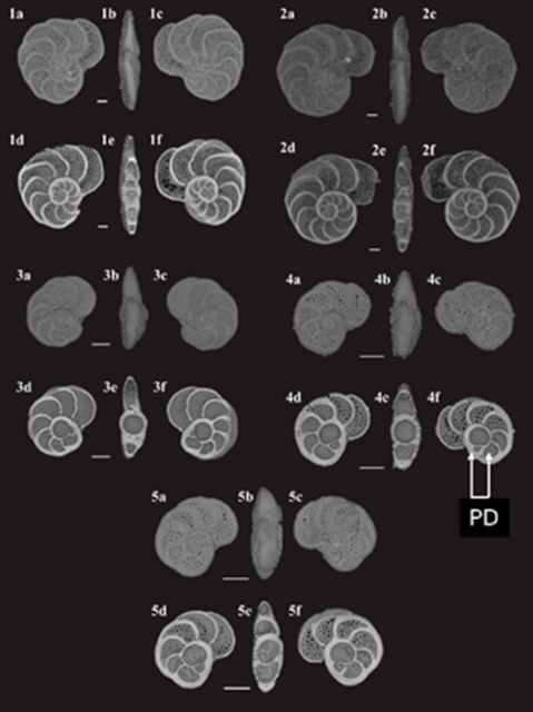
Burkett (2025) reports plastic debris has become a persistent feature of deep-sea ecosystems, yet its role as a habitat for calcifying organisms remains poorly understood. Foraminifera colonization has been observed in significant numbers on plastic surfaces, suggesting that these materials serve as novel and significant deep-sea colonization sites for these abundant calcifying organisms. Her study uses deep-sea experimental plastic substrates to examine the colonization and reproductive morphology of the benthic foraminifera Lobatula wuellerstorfi across three locations. Two sampling locations used OOI platforms on the Oregon continental margin: the Endurance Oregon Offshore site (575 m), and the Regional Cabled Array Southern Hydrate Ridge site (774 m). The third location, Station M (4000 m) was on the abyssal plain off central California. 482 individuals were analyzed for morphometric traits to investigate reproductive morphotypes. One feature examined was the proloculus diameter. The proloculus is the first chamber formed by the foraminifera. In L. wuellerstorfi, the proloculus is the spherical feature visible at the foraminifera center (see Fig. 2, specimen 4f).
The more traditional test morphology of L. wuellerstorfi —characterized by a flattened, biconvex test and consistently elevated and pore-free sutures — is well represented in the Oregon specimens. These samples also displayed a clear bimodal proloculus size distribution, consistent with alternating reproductive strategies, while Station M populations exhibited a broader, less defined bimodal distribution skewed toward megalospheric forms. This variation likely reflects environmentally driven morphologic responses rather than taxonomic divergence. Burkett’s findings demonstrate that plastics can serve as persistent colonization sites for deep-sea foraminifera, offering a unique experimental platform to investigate benthic population dynamics, ecological plasticity, and potential geochemical implications, as well as the broader impacts of foraminifera on deep-sea biodiversity and biogeochemical cycling.
[caption id="attachment_37568" align="alignnone" width="526"]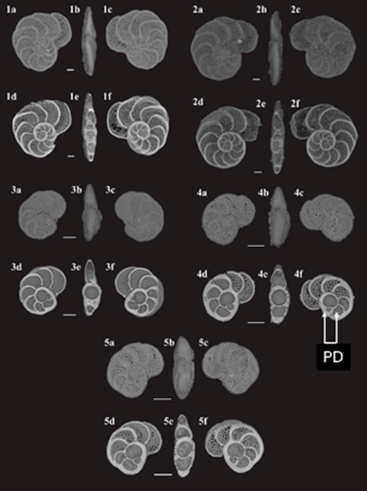 Lobatula wuellerstorfi specimens recovered from plastic substrates at the OOI Endurance Oregon Offshore (575 m water depth) after 264 days of deployment. Each specimen (1–5) is shown in six standardized views for comparative analysis. Specimens 1 and 2 represent microspheric forms; specimens 3–5 are megalospheric individuals that recently completed their first whorl and are smaller in overall test diameter. All scale bars = 100 μm. The proloculus diameter, PD, is indicated on specimen 4f.[/caption]
___________________
Reference:
Burkett, A.M. Life on Plastics: Deep-Sea Foraminiferal Colonization Patterns and Reproductive Morphology. J. Mar. Sci. Eng. 2025, 13, 1597. https://doi.org/10.3390/jmse13081597
Read MoreActive Protothrusts and Fluid Highways: Seismic Noise Reveals Hidden Subduction Dynamics in Cascadia
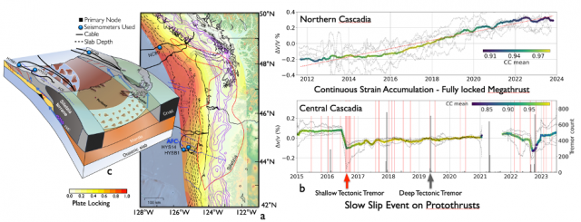
This first of a kind study by Kidiwela et al., (2026) “Active protothrusts and fluid highways: Seismic noise reveals hidden subduction dynamics in Cascadia” (1) applies ambient seismic noise interferometry to a decade of RCA broadband seismometer data at Slope Base and Southern Hydrate Ridge, and on Ocean Networks Canada >400 km to the north at Clayoquot Canyon, to resolve spatio-temporal variations in seismic velocity across the Cascadia Subduction Zone. Along-strike heterogeneity in megathrust behavior, with a strongly coupled (locked) segment in northern Cascadia is in sharp contrast to a weakly coupled central segment characterized by distributed deformation along active protothrusts with slow-slip events. Temporal velocity reductions are suggested to correlate with fluid migration along permeable structures at the plate interface and the subsidiary strike slip Alvin Canyon Fault, indicating that elevated pore-fluid pressures modulate fault mechanical properties. These “fluid highways” facilitate transient weakening and influence stress partitioning, potentially inhibiting the lateral propagation of seismic rupture.
[caption id="attachment_37564" align="alignnone" width="936"]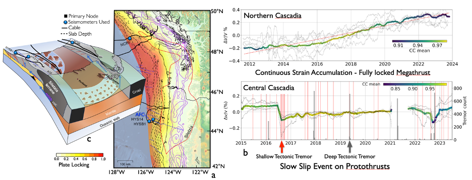 Figure 1 (after Kidiwela Figs 1-3) a) Cascadia Subduction Zone showing a model for the distribution of locking, depth to the down-going slab, strike-slip faults (blue lines) and location of Regional Cabled Array and Ocean Network Canada broadband seismometers used in this study. The Siletzia terrain, a large buried accreted basaltic body is outlined in red. b) Cross sections showing temporal changes in seismic velocities (dv/v) for the Northern and Central Caldera sites. Histograms for shallow (red) and deep (grey) tremor events shown for Central Caldera. c) The cross section shows fluid migration (blue arrows), splay faults and protothrusts (red lines) and the Alvin Canyon Fault (ACF). Down dip tremor, purple dots, match small locked proportions of the slab, Fluid transport along the décollement and the Alvin Canyon Fault are thought to modulate earthquake behavior.[/caption]
The study demonstrates that seismic noise–derived velocity changes provide a sensitive proxy for real-time monitoring of fault zone hydromechanical processes. It provides new constraints on subduction zone segmentation, coupling, and earthquake rupture dynamics and demonstrates a powerful new way to monitor offshore fault zones, ultimately improving our understanding of when and how large earthquakes might occur in Cascadia.
___________________
Reference:
1Kidiwela, M., Denolle, M.A., Wilcock, W.S.D., and Feng, K-F (2026) Active protothrusts and fluid highways: Seismic noise reveals hidden subduction dynamics in Cascadia. Science Advances, 12; https://www.science.org/doi/10.1126/sciadv.aea3684.
Read MoreA Carbon Budget for the Upper Mesopelagic Zone

(Adapted from Stephens et al., 2025)
Upper ocean carbon budgets are difficult to constrain, and those for the mesopelagic zone come with particular challenges. A recent paper by Stephens et al. (2025) took on the challenge of a comprehensive carbon system budget for the upper mesopelagic zone (100-500 m) based on data from the EXport Processes in the Ocean from RemoTe Sensing (EXPORTS) program (Siegel et al., 2016). The 2018 EXPORTS field campaign was conducted at Ocean Station Papa in the Northeast Pacific to take advantage of the relatively modest surface forcing, shallow summer mixed layer, tightly coupled food web, and low mesoscale kinetic energy. Nevertheless, the study found that a steady-state assumption for the carbon system was likely not appropriate.
Measuring organic carbon supply and demand is challenging due to a variety of factors. Supply includes sinking particles, migrating zooplankton and fish, disaggregation, mixing and subduction. Demand comes primarily from bacteria and zooplankton. Measurement methods for each supply and demand term have errors, conversions to rates have uncertainties, and each process being measured may have a unique timescale over which a rate integration makes sense. EXPORTS was notable for increasing the number and variety of measurements available for monitoring the mesopelagic carbon budget. Stephens et al. take advantage of this by combining multiple measurement methods, quantifying errors and applying statistical methods for error analysis.
The authors used observations from multiple sources. Near-surface data came from the PMEL Station Papa surface mooring. Shipboard profile data come from two ships operating during the EXPORTS field campaign as well as the OOI Station Papa cruise in 2018. Additional water column data came from two OOI Slocum gliders, one EXPORTS-operated Seaglider, and BGC Argo floats. The authors examined each carbon supply and demand estimate, calculating an uncertainty and discussing potential limitations (Stephens et al., Table 1). A Monte Carlo approach was used to assess overall uncertainty in supply and demand terms, resulting in the conclusion that supply was insufficient to meet demand (e.g. Fig. 1 below). The error analysis allowed the authors to conclude that the mismatch was not the result of problems in estimating supply or demand, but rather a problem with the assumption that supply and demand would balance within the analysis period. In other words, the system was not in steady state.
This project highlights the complexity of the carbon system in the upper ocean and the broad suite of observational tools necessary to address the carbon budget. The authors make three specific recommendations for improved quantification of the biological carbon pump: including the relevant midwater processes, capturing the range of relevant timescales, and providing redundancy in methodology.
[caption id="attachment_37368" align="alignnone" width="928"]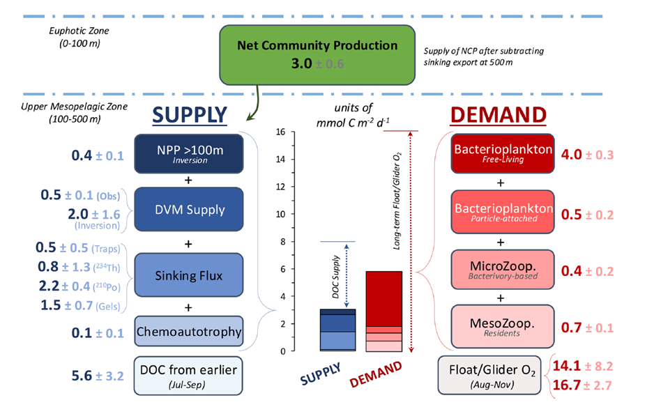 Assessment of the organic carbon budget in the upper mesopelagic zone during EXPORTS. Estimated individual contributions to supply (left) and demand (right) are provided along with error estimates. Terms with multiple measurement methods (far left, far right) were averaged. The center panel shows the cumulative supply and demand relative to a vertical scale in units of mmol C per (m^2 day). From Stephens et al., 2025.[/caption]
___________________
References:
Stephens, B.M., and 20 co-authors, 2025. An upper-mesopelagic-zone carbon budget for the subarctic North Pacific, Biogeosciences, 22, 3301-3328, https://doi.org/10.5194/bg-22-3301-2025.
Siegel, D.A., K.O. Buesseler, M.J. Behrenfeld, C.R. Benitez-Nelson, E. Boss, M.A. Brzezinski, A. Burd, C.A. Carlson, E.A. D’Asaro, S.C. Doney, M.J. Perry, R.H.R. Stanley and D.K. Steinberg, 2016. Prediction of the Export and Fate of Global Ocean Net Primary Production: The EXPORTS Science Plan, Front. Mar. Sci., 3:22, https://doi.org/10.3389/fmars.2016.00022.
Read More
Accounting for Ocean Waves and Current Shear in Wind Stress Parameterization
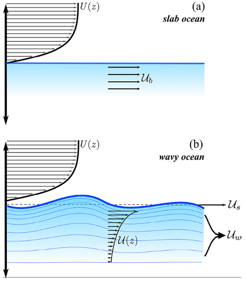
Ortiz-Suslow et al. (2025) use measurements of direct covariance wind stress, directional wave spectra, and current profiles from the OOI Coastal Endurance Array (Ocean Observatories Initiative) offshore of Newport, Oregon (2017–2023) to test a proposed new general framework for the bulk air-sea momentum flux that directly accounts for vertical current shear and surface waves in quantifying the stress at the interface. Their approach partitions the stress at the interface into viscous skin and (wave) form drag components, each applied to their relevant surface advections, which are quantified using the inertial motions within the sub-surface log layer and the modulation of waves by currents predicted by linear theory, respectively.
Their framework does not alter the overall dependence of momentum flux on mean wind forcing, and they found the largest impacts at relatively low wind speeds. Below 3 m s−1, accounting for sub-surface shear reduced form drag variation by 40–50% as compared to a current-agnostic approach. As compared to a shear-free current, i.e., slab ocean, a 35% reduction in form drag variation was found. At low wind forcing, neglecting the currents led to systematically overestimating the form stress by 20 to 50% — an effect that could not be captured by using the slab ocean approach. Their framework builds on the existing understanding of wind-wave-current interaction, yielding a novel formulation that explicitly accounts for the role of current shear and surface waves in air-sea momentum flux. Ortiz-Suslow et al. find their work holds significant implications for air-sea coupled modeling in general conditions.
In using the Oregon Shelf (CE02SHSM) data, Ortiz-Suslow et al. note, “There are several distinct advantages to using these data for this analysis: (1) the range of the dataset goes back seven years with good temporal coverage, (2) there are co-located wind, wave, and current measurements at hourly intervals for in-depth analysis, and (3) the site is exposed to a wide range of wind, wave, and current conditions. Furthermore, by using this dataset, we take advantage of internal quality data control and processing steps that are standardized across the OOI array network.”
[caption id="attachment_37363" align="alignnone" width="488"] Conceptual diagram highlighting the distinction between defining the relative wind velocity over the (a) slab ocean versus the (b) wavy interface. In the presence of near-surface shear, the relative contributions of viscous skin (Us) and wave form (Uw) must be directly accounted when calculating the relative wind at the base of the sheared wind profile (Figure 30, Ortiz-Suslow et al., 2025).[/caption]
___________________
Reference:
Ortiz-Suslow, D.G., N. Laxague, J-V. Björkqvist, M. Curcic, (2025). Accounting for Ocean Waves and Current Shear in Wind Stress Parameterization. Boundary-Layer Meteorology, 191(38), https://doi.org/10.1007/s10546-025-00926-9
Read MoreThe Regional Cabled Array Seen Through the Eyes of Students

One of the OOI’s greatest strengths is its ability to inspire and train the next generation of ocean scientists through immersive, hands-on research at sea and through the analysis and application of large, complex data sets. Students gain authentic, real-world experience in oceanography—working aboard global-class research vessels utilizing advanced robotic vehicles and learning how to communicate their science effectively to broad and diverse audiences. Through the UW VISIONS at-sea experiential learning program more than 200 students have developed these skills while participating in Regional Cabled Array cruises.
Student outcomes are showcased on Interactiveoceans and span an impressive breadth of scientific inquiry. Recent VISIONS’25 projects include short documentaries demystifying hydrophones and distributed acoustic sensing, genetic analyses of deep-sea organisms, and newly developed technologies to probe the metabolomics of life thriving in the extreme environments of hydrothermal vents. These experiences have translated into numerous senior theses with many students presenting their work at professional scientific conferences.
Among the highlights at Ocean Sciences 2026 conference are VISIONS’24–25 student-led presentations that integrated artificial intelligence and computer vision to quantify benthic communities and spatial ecology at Southern Hydrate Ridge. These innovative analyses revealed new connections between biological patterns and methane seep activity, offering fresh insight into the dynamics of this highly active and rapidly changing environment.
[caption id="attachment_37360" align="alignnone" width="445"] RCA Science Highlight: Student Projects and Engagement Products[/caption]
Read More The 2019 marine heatwave at Ocean Station Papa
(Adapted from Kohlman et al., 2024)
Marine Heat Waves (MHW; Hobday et al., 2016) are prolonged periods of extreme ocean sea surface temperature (SST) anomalies. MHWs are typically identified in satellite SST and/or ocean color records; subsurface data and interdisciplinary variables are often lacking. Ocean Station Papa (OSP) provided long-term, interdisciplinary, subsurface data to examine the physical and biochemical characteristics of a MHW in the Northeast Pacific.
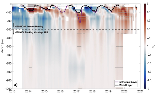
MHWs may have multi-faceted causes, as well as impacts on primary production and higher trophic levels. A recent paper by Kohlman et al. (2024) examines the 2019 NE Pacific MHW using gridded satellite SST data and in-situ observations from multiple OSP platforms including the NOAA Pacific Marine Environmental Lab (PMEL) surface mooring, two OOI Flanking Moorings, the Applied Physics Lab (U. Washington) waverider mooring and shipboard samples from OOI and the Department of Fisheries and Oceans, Canada.
The 2019 MHW was identified in satellite SST data, but the Kohlman et al. study also assessed vertical stratification and the subsurface extent of the temperature signal. The PMEL surface mooring provided temperature and salinity (T/S) down to 300 m. The OOI Flanking Moorings extended the T/S data to 1500 m. The resulting composite time series from 2013-2020 is shown in Fig. 1. Both the extended 2013-2015 MHW and the 2019 MHW are identifiable. Subsurface temperature anomalies during 2013-2014 were strongest above the mixed layer depth (MLD). In the winter and spring of 2017, deeper waters (120–300 m) remained anomalously warm. This anomaly persisted into 2018 due to strong stratification from a fresher surface layer. During the 2019 MHW, anomalously warm waters extended down to 1000 m, whereas the 2013-2015 MHW extended only to about 150 m.
The authors used interdisciplinary data available from Station Papa platforms to assess the drivers and impacts of the 2019 MHW. They found that weaker winds and smaller significant wave height prior to the summer of 2019 created favorable pre-conditioning in the form of an unusually shallow winter MLD. During the MHW, they found that dissolved inorganic carbon and pCO2 decreased, while pH increased. Shipboard samples indicated a decrease in nutrients and an increase in primary productivity. Finally, they speculated that the increased productivity may have had an impact on higher trophic levels – more blue whale calls were recorded in 2019 at Station Papa than normal for Aug-Sep.
This project shows that the characteristics of MHWs are complex. Sustained, multi-disciplinary, subsurface observations are needed to unravel the drivers, pre-conditioning, characteristics, and impacts of these events. Station Papa, among the longest sustained ocean time series sites, is uniquely suited due to the task due to the collaborative observing effort at the site.
[caption id="attachment_37120" align="alignnone" width="512"] Figure 1. Subsurface temperature anomalies at Staton Papa during 2013-2020. Data from the surface to 300 m are from the PMEL surface mooring. Data below 300 m are from the OOI Flanking Moorings. Anomalies are relative to the 1999-2020 Argo climatology. The density-based mixed layer depth (black) and isothermal depth (purple) are overlaid. From Kohlman et al., 2024.[/caption]
___________________
References:
Hobday, A.J., Alexander, L.V., Perkins, S.E., Smale, D.A., Straub, S.C., Oliver, E.C.J., et al. (2016). A hierarchical approach to defining marine heatwaves. Prog. Oceanog., 141(0079–6611), 227–238. https://doi.org/10.1016/j.pocean.2015.12.014.
Kohlman, C., Cronin, M.F., Dziak, R., Mellinger, D.K., Sutton, A., Galbraith, M., et al. (2024). The 2019 marine heatwave at Ocean Station Papa: A multi‐disciplinary assessment of ocean conditions and impacts on marine ecosystems. J. Geophys. Res., 129, e2023JC020167. https://doi.org/10.1029/2023JC020167.
Read MoreSubmarine canyon sediment transport and accumulation during sea level highstand: Interactive seasonal regimes in the head of Astoria Canyon, WA
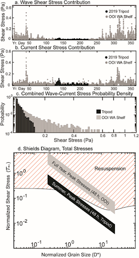
Lahr et al. (2025) use in-situ hydrodynamic data from a benthic tripod deployment in the head of Astoria Canyon to show that sediment resuspension and transport during summer is driven by internal tides and plume-associated nonlinear internal waves. Observations of shoreward-directed currents and low shear stresses (<0.14 Pa) along with sediment trap data suggest that seasonal loading of the canyon head occurs during summer. Nearby long-term wave data from the OOI Washington Shelf mooring shows that winter storm significant wave height often exceeds 10 m, driving shear stress capable of resuspending all grain sizes present within the canyon head. Swell events are generally concurrent with downwelling flows, providing a mechanism for episodic downcanyon sediment flux. This study indicates that canyon heads can continue to function as sites of sediment winnowing and bottom boundary layer export even with a detached, shelf-depth canyon head.
As part of this study, Lahr et al. (2025), used data from the OOI Washington Shelf Surface Mooring located 81 km north of the tripod site in Astoria Canyon. The 2019 benthic tripod deployment by Ogston was done as an ancillary activity on the Endurance 11B cruise aboard R/V Oceanus. The data used were concurrent spectral surface wave and meteorological data near bed current velocity for 2016 (chosen for its complete records). Figure xx shows the benthic tripod stress overlaid with the OOI Washington shelf mooring stress. Over the summer, the benthic tripod stress and OOI estimated stress compare well. Winter stresses (available from OOI mooring only) are much larger than those observed in summer.
[caption id="attachment_37116" align="alignnone" width="277"] Figure 1. Shear stress computed from the Astoria Canyon tripod deployment (black) and the OOI Shelf mooring (gray). Panels a) and b) depict relative stress contributions from waves and currents respectively, c) the distribution of total stresses, and d) maximum shear stresses from summer and winter on a Shields diagram. (Figure 3, Lahr et al., 2025)[/caption]
___________________
Reference:
Lahr, E.J., A.S. Ogston, J.C. Hill, H.E. Glover, and K.J. Rosenberger (2025). Submarine canyon sediment transport and accumulation during sea level highstand: Interactive seasonal regimes in the head of Astoria Canyon, WA. Marine Geology, no. (2025): 107516. https://www.sciencedirect.com/science/article/pii/S0025322725000416.
Read MoreRCA Broadband Provides First Report of Tremor-Like Signals Offshore Cascadia
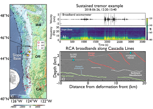
The recent publication “Possible Shallow Tectonic Tremor Signals Near the Deformation Front in Central Cascadia” (Krauss et al., 2025) presents the first report of tectonic tremor-like signals offshore Cascadia. As described by the authors, deep slow-slip events in Cascadia—lasting from hours to weeks—have been documented by land-based stations for decades. These events can accommodate a significant portion of overall plate motion and may serve as precursors to megathrust earthquakes. Over the past two decades, significant tectonic tremor activity (1–10 Hz) has been observed as a feature of slow slip every 10.5–15.5 months beneath Vancouver Island to northern Oregon (Bombardier et al. 2024), with annual slip events equivalent to a magnitude ~6.5 earthquake. These typically occur well inland, at depths of approximately 30–40 km. Contrastingly, it is unknown whether slow-slip events and accompanying tectonic tremor occur at shallow subduction depths in the offshore region.
Krauss et al. (2025) analyzed data collected 2015-2024 from buried ocean-bottom seismometers (OBS) at two sites: Slope Base (2,920 m depth), located 5 km seaward of the deformation front, and Southern Hydrate Ridge (790 m depth), approximately 20 km landward. The analysis incorporated in-situ bottom current data. After applying short- and long-term averaging techniques, the study identified 85,000 signals at Slope Base and 30,055 at Southern Hydrate Ridge, encompassing T-phase events, ship noise, and tectonic tremor-like signals. Notably, tectonic tremor-like signals were observed exclusively at Slope Base.
These signals cannot be attributed to ship traffic or environmental noise. Instead, they are hypothesized to originate from slow slip on one of many nearby tectonic structures: the décollement fault, faults near the subduction zone front and outermost accretionary wedge, faults on the incoming Juan de Fuca Plate, or nearby strike-slip structures such as the Alvin Canyon Fault. However, without additional observations of these signals on multiple stations, it is unclear whether they are tectonic or represent another signal altogether.
Future deployments, such as those planned through the Cascadia Offshore Subduction Zone Observatory (COSZO) will improve our ability to pinpoint the sources of these offshore tremors. The full dataset and results are available on GitHub (https://github.com/zoekrauss/obs_tremor) and archived on Zenodo (https://zenodo.org/records/14532861).
[caption id="attachment_37111" align="alignnone" width="512"] Figure 1. a) Location of the Regional Cabled Array cabled broadband seismometers (OBS’s -cyan triangles) offshore Newport Oregon and an autonomous instrument (purple triangle), earthquakes (pink circles) and along and just offshore the Cascadia Margin. b) sustained tremor-like signals from the broadband at Slope Base. c) Subsurface structure across strike of the margin showing location of Slope Base and Southern Hydrate Ridge OBS’s, accretionary margin faults and demarcation of a boundary interpreted to be a protothrust between the sedimentary column and the incoming Juan de Fuca Plate crust.[/caption]
___________________
References:
Krauss, Z., Wilcock, W.D.S., and Creager, K.C. (2025) Possible shallow tectonic tremor signals near the deformation front in Central Caldera. Seismica, https://seismica.library.mcgill.ca/article/view/1540.
Bombardier, M., Cassidy, J.F., Dosso, S.E., and K. Honn (2024) Spatial distribution of tremor episodes from long-term monitoring in the northern Cascadia Subduction Zone. Journal of Geophysical Research, https://doi.org/10.1029/2024JB029159.
Read MoreSAR Imagery Detects Atmospheric Stratification
(Adapted from Stopa et al., 2024)
There is interest in using satellite-based Synthetic Aperture Radar (SAR) imagery to assess phenomena related to atmospheric boundary layer stratification over the ocean. Obtaining such information with high spatial and temporal resolution would advance boundary layer research and would be beneficial to the development of offshore wind energy. However, monitoring marine boundary layer structure remotely is a challenge. A recent paper by Stopa et al. (2024) shows that it is possible to utilize SAR imagery, in conjunction with in-situ meteorology, to characterize boundary layer stratification.
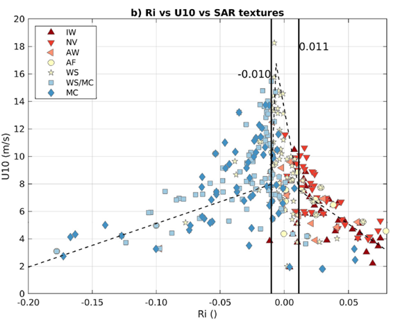
The Central Surface Mooring (CNSM) of the OOI Pioneer New England Shelf Array is located near a region of offshore wind development where SAR imagery is also available. The authors use wind speed, air temperature, and sea surface temperature from the CNSM buoy to estimate the bulk Richardson number (Ri), a measure of marine atmospheric boundary layer stability. OOI quality control flags were used to identify good data, and suspect data were replaced with data from redundant sensors. CNSM data from 2014 – 2021 were used in the analysis.
SAR data are commonly used to provide wind speed estimates, but the images also contain rich information about coherent structures in the atmosphere, and those structures correspond to boundary layer stratification regimes (Stopa et al., 2022). The Stopa et al., (2024) study used European Space Agency Sentinel-1 C-band SAR wave mode (S1 WV) imagery spanning the region of the NES Pioneer Array. SAR Images in 20 x 20 km regions were visually examined and classified based on observed “signatures” of atmospheric phenomena. Of particular interest for this study were signatures indicative of waves, rolls/streaks and convection (Table 1).
The relationship of SAR image classes to wind speed and atmospheric stability was examined by plotting the classified data set vs Ri and U10 (Figure 1). U10 shows a change in slope near neutral stratification (Ri = 0) with indications of a Ri-U10 relationship at higher and lower Ri. Of interest is the appearance of Ri boundaries denoting transitions between unstable (Ri < -0.01), neutral, and stable (Ri > 0.01) regimes. Rolls, streaks and convection dominate the unstable regime, while waves dominate the stable regime. In other words, classification of the SAR images provides information about atmospheric stratification.
This project shows the power of combining remote sensing with long-term, in-situ meteorological measurements to gain insights that neither could provide alone. The authors note that when satellite data are available, the SAR-based determination of boundary layer structure can be used over broad areas and long times, and is more efficient than direct measurements such as buoy-based LIDAR.
Table 1: Atmospheric signatures in SAR imagery
| Class | Phenomena |
| NV | Lack of rolls or cells |
| AW | Atmospheric gravity waves |
| IW | Oceanic internal gravity waves |
| WS | Rolls or wind streaks |
| MC | Microscale convection |
| WS/MC | Combined WS/MC |
Figure 1. SAR image classes shown as different symbols) vs. Richardson number (Ri) and ten meter wind speed (U10). Note the regime transitions near Ri = -0.01 and +0.01. From Stopa et al., 2024.[/caption]
___________________
References:
Stopa, J.E., C. Wang, D. Vandemark, R.C. Foster, A. Mouche, and B. Chapron, (2022). Automated Global Classification of Surface Layer Stratification Using High-Resolution Sea Surface Roughness Measurements by Satellite Synthetic Aperture Radar,” Geophysical Research Letters 49(12), e2022GL098686.
Stopa, J.E., D. Vandemark, R. Foster, M. Emond, A. Mouche, and B. Chapron (2024). Characterizing the Atmospheric Boundary Layer for Offshore Wind Energy Using Synthetic Aperture Radar Imagery. Wind Energy, 27:1340–1352, https://doi.org/10.1002/we.2933.
Read More