
Data
Four-Part Series on Using Data Explorer
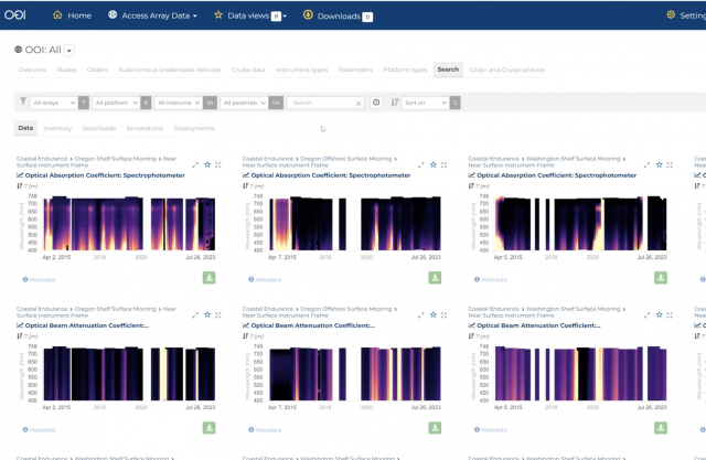
OOI Data Specialist Stace Beaulieu has put together a four part-series demonstrating how to use Data Explorer. In eight minutes or less per session, you can learn how to find and visualize time-series, glider, or profiler data and compare time-series data. The demos can be accessed below, on YouTube, and permanently under Tutorials on this website. Be sure to bookmark the site for future reference. A print version of the four-part series can be accessed and downloaded here.
[embed]https://youtu.be/9CA5GsGL2-0[/embed] [embed]https://youtu.be/SEwHMSyQFUg[/embed] [embed]https://youtu.be/smrSszcO4RY[/embed] [embed]https://youtu.be/ql8JvTGyrmI[/embed] Read MoreNew Features of Data Explorer Demo
In case you missed it, here is a video of the OOI Town Hall on July 26, 2023 during which the new features of Data Explorer were demonstrated and questions answered.
[embed]https://vimeo.com/849129117[/embed] Read MoreEfforts to Standardize Data Continue
The OOI Data Teams have recently made great strides in ongoing efforts to standardize data, making it easier for users to understand what OOI data and metadata are available. Efforts have focused on improving labeling, descriptions, and correcting units to ensure consistency. A major improvement underway is matching variable naming conventions with those governed by Climate and Forecast (CF) metadata standards.
The first round of changes is expected to be completed by the end of June 2022. Once these changes are implemented, existing scripts used to download and process OOI data files could be impacted depending on how the code was written. The Data Teams will publish a list of affected streams and recommended code updates prior to the release of these changes, to highlight the improvements and to allow for processing script modifications.
Read MoreOOI Data System User Survey: Opportunity to Provide Feedback
The OOIFB Data Systems Committee needs your help in evaluating new Ocean Observatories Initiative (OOI) data systems. In 2019 the OOI Facility Board’s Data Systems Committee (DSC) conducted a survey to learn how the OOI could better serve data to users. In response to the feedback received, the OOI program developed the Data Explorer, a refined and more capable interface for finding and accessing data. Now, the DSC is interested to hear your thoughts on this new data system, as well as the other available systems, and to uncover potential ways of improving data access for users.
Near Real-time CTD Data from Irminger 8 Cruise (August 2021)
In August 2021, members of the OOI team aboard the R/V Neil Armstrong for the eighth turn of the Global Irminger Sea Array and members of OSNAP (Overturning in the Subpolar North Atlantic Program) onshore are making near-real time shipboard CTD data available.
Onshore expert hydrographer, Leah McRaven (PO WHOI) from the US OSNAP team, is working with the shipboard team to support collection of an optimized hydrographic data product. A special feature of this collaboration is the near real-time sharing of OOI shipboard CTD data with the public. Interested parties will have access to the same CTD profiles that McRaven will be reviewing.
McRaven is sharing her reports here while the cruise is underway:
BLOGPOST #4 (September 13, 2021)
Another OOI cruise is in the books! Now that things have wrapped up and I’ve had a chance to dig into the data a bit more thoroughly, how did we do? In my previous post I reported that the Irminger 8 CTD data looked to be very promising, but I like to include one more step before recommending data to be used for science: carefully considering salinity bottle data.
Salinity bottle data can be used in many ways to support a particular scientific objective or research question. The two that I’ve become most familiar with are 1) to support the analysis of additional bottle samples (e.g. dissolved oxygen) and 2) to provide an additional assessment and calibration of the CTD conductivity sensors. Both applications are necessary when researchers require salinity values more accurate than what CTD sensors are able to provide. However, even if this is not required, it can help ensure that users receive data that are reasonably within manufacturer specifications.
I find it easiest to consider the GO-SHIP approach to bottle data first. Using ship-based hydrography, GO-SHIP provides approximately decadal resolution of the changes in inventories of heat, freshwater, carbon, oxygen, nutrients, and transient tracers, covering the ocean basins with global measurements of the highest required accuracy to detect these changes. For a program like this, 36 salinity samples are taken every CTD station in order to provide an extremely accurate and precise calibration for the CTD sensors. Interestingly, the Irminger OOI array is bracketed by three GO-SHIP repeat transects. While GO-SHIP provides invaluable measurements, drawing a large number of samples can be expensive and time consuming. Additionally, measurements occur on a decadal timescale, so there is a lot of the picture we miss.
One of the research programs that aims to provide a higher temporal and special resolution picture of the North Atlantic is OSNAP. This program has several scientific objectives, but generally aims to quantify intra-seasonal to interannual variability of the Atlantic Meridional Overturning Circulation(AMOC) in the subpolar Atlantic. This includes a focus on heat and freshwater fluxes, pathways of currents throughout the region, and air-sea interaction, all of which require highly calibrated data products. In order to accomplish this, PIs from the program need to be able to consistently merge their shipboard and moored data products for cohesive and accurate quantification of parameters. Because much of the variability being studied is so large, researchers do not necessarily need salinity accuracies at the level of GO-SHIP, but they do need to use salinity bottle samples to ensure that CTD casts are at the very least within manufacturer specifications.
In the end, no one approach to hydrographic sampling is necessarily better than another. What is important is the delicate balance of resources while at sea that best support the scientific objectives. For both OSNAP and OOI, where the primary work at sea is focused on servicing moorings, the resources for a GO-SHIP approach to sample bottle collection is simply not feasible. However, one very key feature of the OOI CTD data is that they are collected annually, while ONSAP data are collected every two years, and GO-SHIP data are collected every ten years. Hence, OOI is able to fill in some of the temporal data gaps in the region and greatly bolster many of the international programs working in the region.
This year OOI collaborated with numerous PIs and representatives from research programs that operate in the Irminger Sea region to produce a more optimized CTD and bottle sampling strategy that better complements goals similar to GO-SHIP, as well as several additional objectives from international programs, such as OSNAP. The goal of this updated plan was to provide OOI data end users and collaborators with data that are more appropriate for CTD, mooring, glider, and float instrumentation calibration purposes. In particular, the update included increased sampling of the deep ocean. Such data are critical in the Irminger Sea region due to the uniquely large variability of temperature, salinity, and chemical properties throughout the shallow and intermediate depths of the water column. Deeper CTD and bottle data will allow all end users to more carefully reference their scientific findings to more stable water masses and allow for better intercomparison with other available datasets, such as the available GO-SHIP and OSNAP data from the region.
The majority of methods that I use when considering salinity bottle data have been adapted from GO-SHIP and NOAA/PMEL. In particular, many of the cruises I work with, including OOI, often have far fewer bottle samples than recommended by GO-SHIP or PMEL methods. This isn’t necessarily bad, since we don’t need to achieve the same goals as those programs, however, great care in adapting methods does need to be considered (and I encourage you to reach out if this is something you have an interest in). So, with the improved OOI sampling scheme, what are the potential benefits to CTD data quality?
More strategically planned salinity bottle sample collection allows users to:
- Decide if data from primary or secondary sensors are more physically consistent
- Identify times when CTD contamination was not obvious
- Assess manufacturer sensor calibrations
- Potentially provide a post-cruise calibration
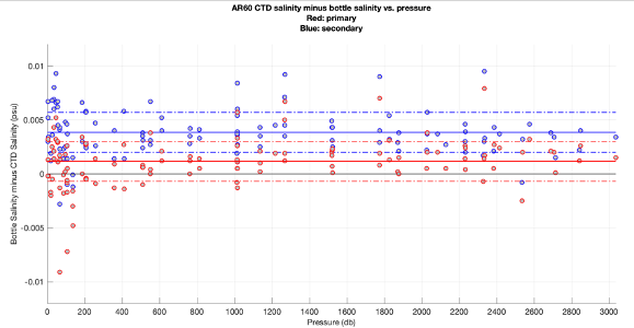
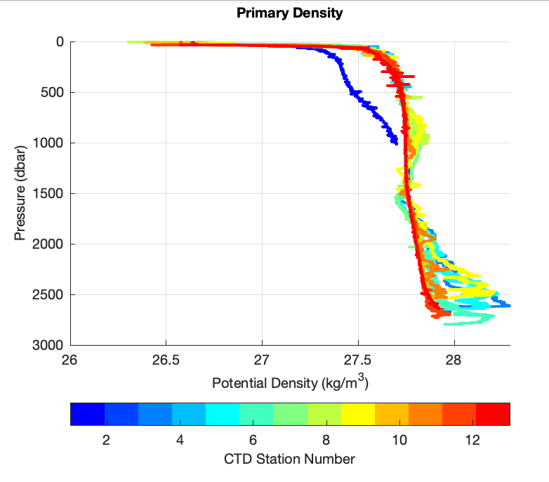
In the case of the Irminger 8 cruise, I see that all four uses of salinity bottle data are possible, which will make a lot of collaborators very happy! Starting with Figure 1, we can see a summary of CTD and bottle sample salinity differences as a function of pressure for both the primary and secondary sensors. As a rule of thumb, the average offset of these differences can be considered an estimate of sensor accuracy, and the spread, or standard deviation, can be considered an estimate of sensor precision. While the data have a fairly large spread to the eye, the standard deviations (indicated by the dashed lines) are placing the spread for each sensor within what we expect from the manufacturer precision. The striking result from this figure is that before using the bottle data to further calibrate the data, we see that the primary sensor had a higher accuracy than the secondary sensor. In going back to the Seabird Electronics calibration reports for the primary and secondary sensors (available via the OOI website), I noted that the calibrations for each sensor was a bit older than what we normally work with (last performed in May 2019). Additionally, the secondary sensor had a larger correction at its time of manufacturer calibration than the primary. This is corroborated by the differing sensor accuracies as determined by the bottle data. Lastly, while there are a few spurious differences shown, on average there doesn’t look to be any CTD and bottle differences due to factors other than expected calibration drifts.
Figure 1
In order to apply a calibration based on the bottle data to the CTD data, I first QC’d the bottle data and then followed methods described in the GO-SHIP manual. There are several sources of error that can contribute to incorrect salinity bottle values, ranging from poor sample collection technique to an accidental salt crystal dropping into a sample just before being run on a salinometer. This is why all methods of CTD calibration using bottle data stress the importance of using many bottle values in a statistical grouping. However, sometimes there are “fly-away” values that are so far gone they don’t contribute meaningful information to the statistics, and in those cases I simply disregard those values. As a reference, for the Irminger 8 cruise I threw out 9 of the ~125 salinity samples collected before proceeding with calibration methods. Note that within the methods described in the above documentation, systematics approaches are used to further control for outlier or “bad” bottle values.
Figure 2
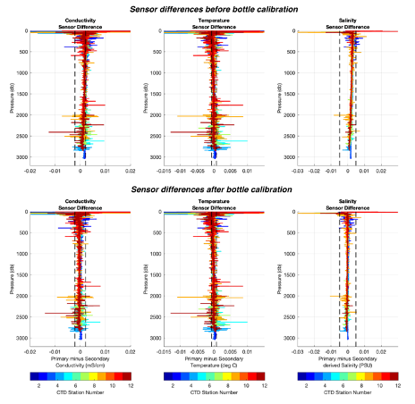
Since the majority of CTD stations for OOI are performed close to one another (and consequently in similar water masses), I grouped all stations together to characterize sensor errors. The resulting fits produced primary and secondary sensor calibrations that allow for more meaningful comparison of data with other programs. Figure 2 shows how primary and secondary data compare before and after bottle calibrations have been applied. Post calibration, primary and secondary sensors now agree more closely in terms of their differences. Similarly, Figure 3 summarizes data before and after calibration in temperature-salinity space, providing visual context for the magnitude of bottle calibration. Many folks working with CTD data would say that this is a rather small adjustment!
Figure 3
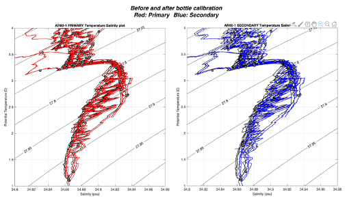
Figure 4
 However, Figure 4 shows a comparison of the bottle-calibrated OOI data with nearby OSNAP CTD profiles from 2020. The results here are extremely important as OSNAP currently has moorings deployed near the OOI array and the OOI CTD profiles provide a midway calibration point for the moored instrumentation that is currently deployed for two years. These midway calibration CTD casts are critical in providing information on moored sensor drift and biofouling in a region where there has been a slow freshening of deep water (colder than 2.5 ºC) throughout the duration of these programs. Quantifying the rate of freshening is one of the objectives that OSNAP focuses on, but it is nearly impossible without high-quality CTD data for comparison. Figure 4 demonstrates that the freshening trend has continued from 200 to 2021 and that the bottle-calibrated OOI CTD data will be critical for interpretation of moored data.
Finally, for those interested in the salinity-calibrated CTD dataset, please contact lmcraven@whoi.edu. A more detailed summary of the calibration applied can be found in my CTD calibration report here.
BLOGPOST #3 (August 18, 2021)
Irminger 8 science operations are now fully underway, which means the stream of CTD data is coming in hot (actually the ocean temps are very cold)! So far, CTD stations 4 through 11 correspond to work performed near the Irminger OOI array location. I spent the weekend and past couple of days paying close attention to these initial stations. Here’s an update on how things look so far.
One of the concerns this year is that the R/V Neil Armstrong is using a new CTD unit and sensor suite (new to the ship, not purchased new). Any time a ship’s instrumentation setup changes, it’s a very good idea to keep a close eye on things as changes naturally mean there’s more room for human error. What better way to talk about this than to share my own mistakes in a public blog! When I first downloaded and processed the OOI Irmginer 8 (AR60) CTD data from near the Irminger OOI array location, I became very worried…
When I compared the Irminger 8 CTD data with three cruises from the same location last year, I was seeing very confusing and unphysical data in my plots. I was using Seabird CTD processing routines in the “SBE Data Processing” software (see https://www.seabird.com/software) that I had used for previous OOI Irminger cruises as a preliminary set of scripts, so I was confident that something strange with the CTD was going on. I immediately pinged folks on the ship to ask if there was anything that they could tell was strange on their side of things. Keep in mind, this OOI cruise focuses more on mooring work with only a handful of CTDs to support all additional hydrographic work, so any time there is a potential issue with the CTD data we want to address it as soon as possible. I started digging into things a bit more, and realized that I had made a mistake.
Within the SBE processing routines, there is a module called “Align CTD”. As stated in the software manual: “Align CTD aligns parameter data in time, relative to pressure. This ensures that calculations of salinity, dissolved oxygen concentration, and other parameters are made using measurements from the same parcel of water. Typically, Align CTD is used to align temperature, conductivity, and oxygen measurements relative to pressure.” When working in areas where temperature and salinity change rapidly with pressure (depth), this module can be very important (and I encourage you to read through its documentation). As you’ll see below, the OOI Irmginer Sea Array region can see some extremely impressive temperature and salinity gradients. This has to do with the introduction of very cold and very fresh waters from near the coast of Greenland, together with the complect oceanic circulation dynamics of the region. Based on data collected on the old CTD installed on the Armstrong, I had determined that advancing conductivity by 0.5 seconds produced a more physically meaningful trace of calculated salinity.
While 0.5 seconds doesn’t seem large, it’s important to remember that most shipboard CTD packages are lowered at the SBE-recommended speed of 1 meter/second. Depending on how suddenly properties change as the CTD is lowered through the water, this magnitude of adjustment may seriously mess things up if it’s not the correct adjustment. In the case of the CTD system currently installed on the Armstrong, I’m finding that very little adjustment to conductivity is needed. There are many reasons as to why this value will change – from CTD to CTD, cruise to cruise, and even throughout a long cruise. The major factor is the speed at which water flows through the CTD plumbing and sensors and how far the pressure, temperature, and conductivity sensors are from each other in the plumbed line. Water flow is controlled by many things including CTD pump performance, contamination in the CTD plumbing, kinks in the CTD pluming lines, etc. (for more information, start here: https://www.go-ship.org/Manual/McTaggart_et_al_CTD.pdf and here: file:///Users/leah/Downloads/manual-Seassoft_DataProcessing_7.26.8-3.pdf. Note that the SBE data processing manual provides great tips on how to choose values for the Align CTD module.
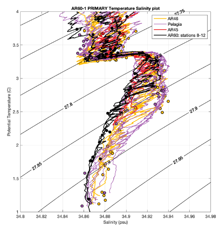
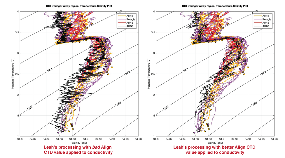
Below is a figure that summarizes impact on my processed data before and after my mistake. This is a fun figure as it compares CTD data from four cruises that all completed CTDs near the OOI site: the 2020 OSNAP Cape Farewell cruise (AR45), the 2020 OOI Irminger 7 cruise (AR46), a 2020 cruise on R/V Pelagia from the Netherlands Institute for Sea Research, and stations 5-7 of the 2021 OOI Irminger 8 cruise (AR60). I’m plotting the data in what is called temperature-salinity space. This allows scientists to consider water properties while being mindful of ocean density, which as mentioned in the last post, should always increase with depth. I include contours indicating temperature and salinity values that correspond to lines of constant density (in this case I am using potential density referenced to the surface). For data to be physically consistent, we expect that the CTD traces never loop back across any of the density contours. These figures are also incredibly useful as the previous three cruises in the region give us some understanding of what to expect from repeated measurements near the Irminger OOI array.
The plot on the left shows the data processed with a conductivity advance of 0.5 sec. As you can see, the CTD traces appear much noisier than the other datasets, and contain many crossings of the density contours (i.e., density inversions). The plot on the right shows data that are smoother and less problematic in terms of density. You may also note that in the right plot, the AR60 traces are a bit shifted to the left in salinity (i.e. fresher or lower salinity values) when compared to the other datasets. This is because I am plotting bottle-calibrated CTD data from the other three cruises. Just as I type this, I’ve been given word that the shipboard hydrographer has begun analyzing salinity water sample data for Irminger 8. These bottle data are critical for applying a final adjustment to CTD salinity data and I’ll talk more about this in a future post.
For now, I’m happy to report that the data look physically consistent! For completeness, I include the core CTD parameter difference plots from stations 4 through 11 (CTDs completed near the array thus far). CTD difference plots are described in my previous post. All checks out from where I am sitting so far. Thanks to the CTD watch standers and shipboard technicians for working so hard and taking good care of the system while the cruise is underway!
BLOGPOST #2 (August 10, 2021)
For this post I’d like to introduce some of the tools that folks can use to identify CTD issues and sensor health while at sea. Most of what I’ll be discussing here is specific to the SBE911 system that is commonly used on UNOLS vessels; however, a lot of these topics are relevant to other types of profiling CTD systems.
There are several end case users of CTD data within science. These include people who perform CTDs along a track and complete what we call a hydrographic section (useful in studying ocean currents and water masses); those who perform CTDs at the same location year after year to look for changes; people who use CTDs to calibrate instrumentation on other platforms (moorings, gliders, AUVs, etc.); and those who use the CTD to collect seawater for laboratory analysis (collected samples can be used to further analyze physical, chemical, biological, and even geological properties!). For each of these CTD uses, a core set of CTD parameters are needed.
Core CTD parameters include pressure, temperature, and conductivity. Conductivity is used together with pressure and temperature measurements to derive salinity. These three variables are needed to give users the critical information of depth and density in which water samples are collected, and support the calculation of additional variables. For example, ocean pressure, temperature, and salinity together with a voltage from an oxygen sensor are needed to derive a value for dissolved oxygen. In addition to core CTD parameters, it is very common to add dissolved oxygen, fluorescence, turbidity, and photosynthetically active radiation (PAR) sensors to a shipboard CTD unit. Each of these additional measurements have errors that must be propagated from the core CTD measurements – creating a rather complex system to navigate when trying to understand the final accuracy of a given measurement.
For each CTD data application, varying degrees of accuracy are needed from the measured CTD parameters to accomplish the scientific objective at hand… And this is where a lot of folks get into trouble! For a first example, consider someone who would like to calibrate a nitrate sensor that is deployed for a year on a mooring using water samples collected from the CTD. For a second example, consider someone who is interested in the changing dissolved oxygen content of deep Atlantic Meridional Overturning Circulation waters. In both cases, the core CTD parameters are critical. In the first example, this person needs to know the pressure and ocean density at the exact location their water samples are collected during a CTD cast so they can correctly associate analyzed water sample values with the correct position of the sensor on the mooring. However, in the second example, this person may need to use both salinity and oxygen samples to improve the accuracy and precision of CTD measurements so that their final data product will be sensitive enough to resolve small, but potentially critical, changes in the ocean.The most important take away here (CTD soapbox moment!) is that even if end users are not specifically interested in studying physical oceanographic parameters, they still need tools to verify that 1) the core CTD measurements are of high enough quality for use in their application and 2) that there are no unnecessary errors from the core measurements that are impacting their ability to address their scientific objective.
This is the first reason why I heavily encourage all CTD end users to become familiar not only with the accuracy of their particular measured parameter, but also the core CTD parameters. The second reason is that core CTD parameters are particularly useful in diagnosing early warning signs of CTD problems. Most shipboard systems install primary and secondary temperature and conductivity sensors on their CTDs, which provide an opportunity for in-situ sensor comparison. Additionally, calculated seawater density is particularly useful as it is one of the few properties we can make a strong assumption about – it should always increase with pressure. The density of seawater is determined by pressure, temperature, and salinity (conductivity), hence any time one or some of these recorded values is suspect, non-physical density “inversions” or “noise” may appear in the data record.
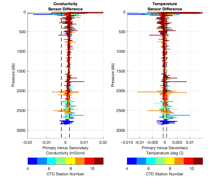
Below are two figures that can be very helpful in diagnosing CTD problems. In these examples, I am using the Irminger 8 (AR60-01) deep test cast, which took place late Sunday evening, August 8th. Figure 1 shows difference plots of the two sensor pairs (temperature and conductivity). Each panel includes vertical dashed lines indicating expected manufacturer agreement ranges (see sensor specification sheets datasheet-04-Jun15.pdf and datasheet-03plus-May15.pdf). The values shown are, ±(2 x 0.001 ºC) and ±(2 x 0.003 mS/cm) for temperature and conductivity sensors, respectively (note that 0.003 mS/cm is close to 0.003 psu for reasonable temperature ranges). In general, sensor differences should fall within, or very close to, this range when calibrated by the manufacturer within the past year. The rule can be relaxed in the upper water column, however, differences between sensors deeper than approximately 500 m that consistently fall outside of this range indicate problematic sensor drift or contamination. Figure 2 shows the calculated seawater density profile using the primary sensors. Consistent density inversions larger than ~0.1 kg/m3 also indicate problematic sensor drift or contamination. When creating such figures, always look at the downcast and upcast (skipped here for the sake of brevity). The upcast will look a bit worse than the downcast (I encourage you to read about why), but those data are extremely important to anyone collecting water samples!
Figure 1
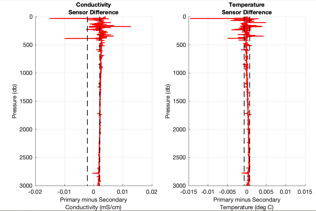
Figure 2
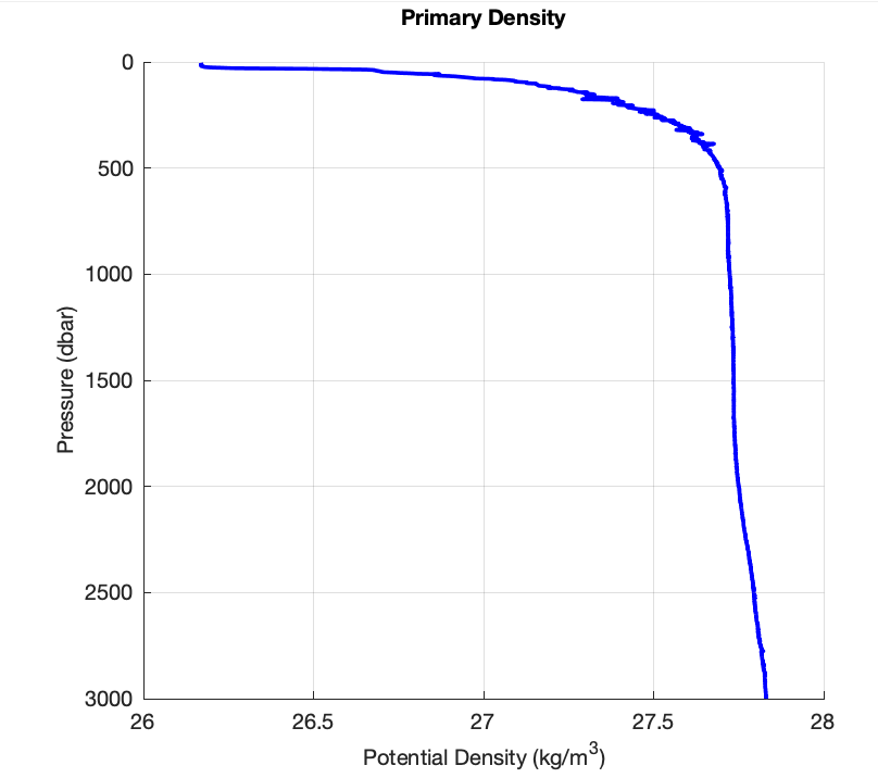
So, what can these plots tell us about the CTD system implemented on the Irminger 8 cruise so far? Figure 1 demonstrates an overall acceptable level of agreement between the sensor pairs. The particular sensors in use right now have calibrations older than one year, so this level of agreement is actually quite good. Figure 2 is also rather promising in showing a density profile that is continuously increasing. If you’re being picky (like me), you may notice that there are some small density inversions between roughly 200-500 m. After taking a closer look, I noted that the salinity profile indicates that there are some rather impressive salinity intrusions evident in the upper 500 meters (I encourage you to download data from cast 2 and verify!). This is normal for the Labrador Sea region where the cast took place (lots of melting ice nearby) and will naturally create a bit more “noise” in these plots. So, I’m not very concerned by this.
Now what do these plots look like when there’s a problem? There unfortunately isn’t one simple answer for this (I’ve been doing this for over ten years and am still learning subtle ways CTDs show problems!), but I’ll share two examples of when something was clearly wrong. The first example is from the Irminger 7 cruise (AR35-05). Figure 3 and Figure 4 show our two plots for stations 1-13 of the Irminger 7 cruise. Figure 3 shows a suspiciously large offset (well outside of the general threshold we expect in the conductivity differences) and incredibly noisy differences in both conductivity and temperature. Similarly, Figure 5 shows consistent and large density inversions for some of these casts. Several of the casts shown in Figures 4 and 5 were so bad that there are no usable profiles as far as scientific objectives are concerned. Luckily, however, there were a few casts in the set that could be corrected with water sample data (I’ll talk more about this later). Data loss is something that does happen while at sea, and the Irminger Sea in particular is an incredibly harsh environment to work in. However, if folks are diligent in creating these plots while at sea, the hope is that we can minimize time and data loss while striving for the highest quality data possible.
Figure 3
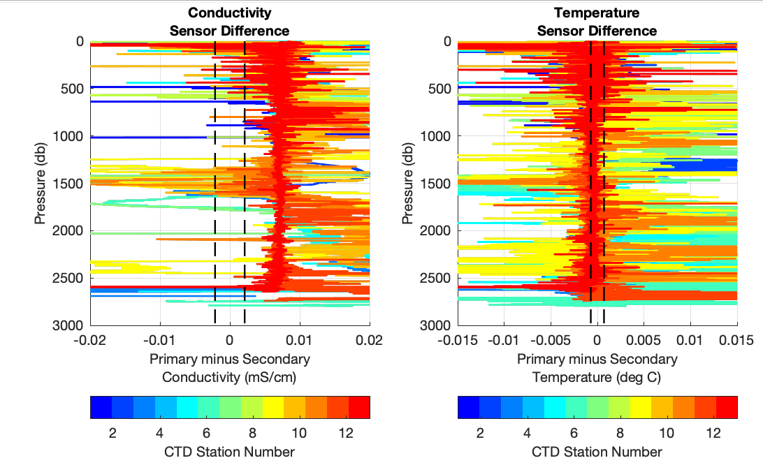
Figure 4
For my last example, I provide a quick reference guide for how core CTD parameter issues may look on a Seabird CTD Real-Time Data Acquisition Software (Seasave) screen. The reason for this is that a lot of people don’t have time to create fancy plots while at sea, so it’s helpful to know how to approach monitoring while watching the data come in. Follow the link here to download a one-page pdf that can be displayed next to your CTD acquisition computer.
BLOG POST #1 (August 2, 2021)
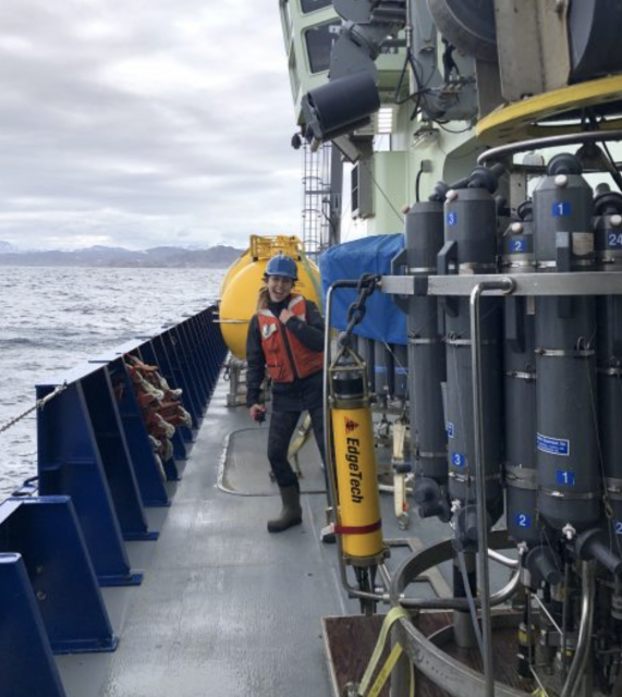
[caption id="attachment_21736" align="aligncenter" width="2560"]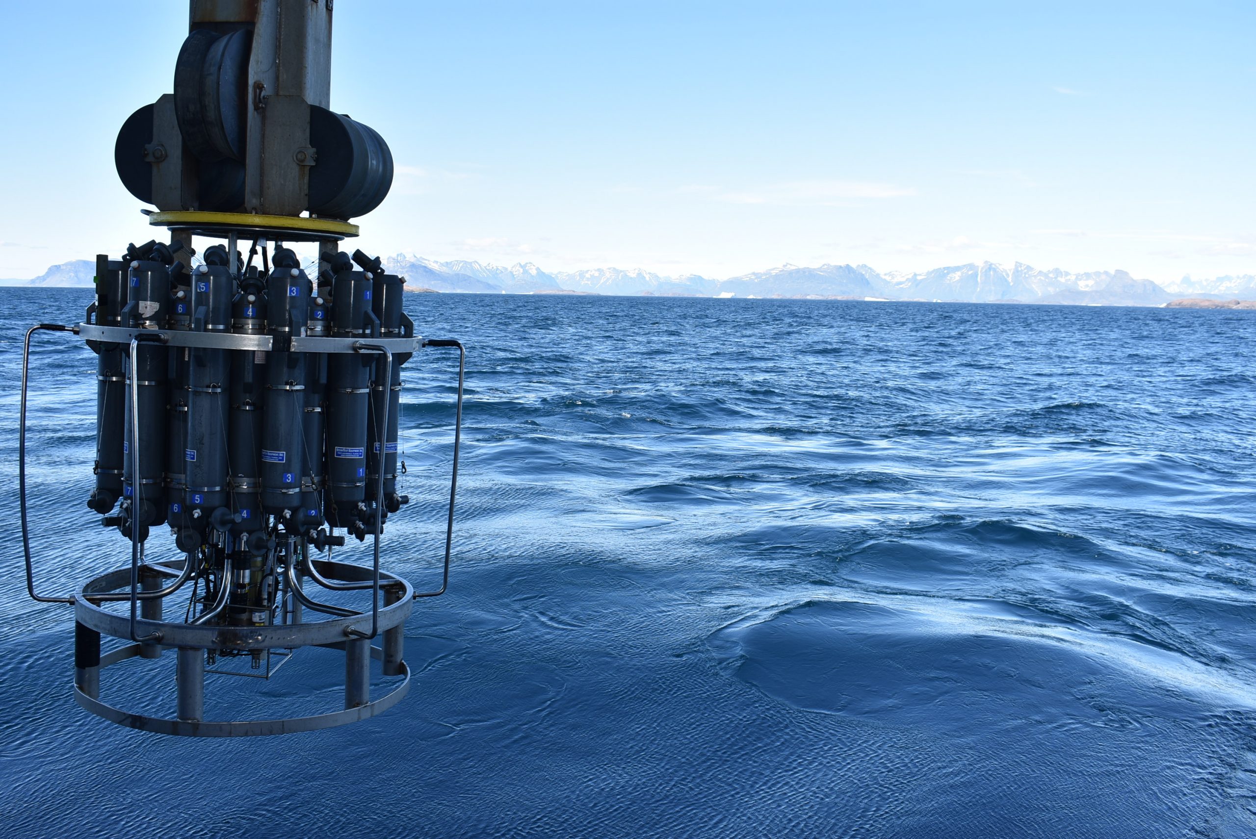 A CTD is performed near the coast of Greenland during one of the OSNAP 2020 cruises on R/V Armstrong. Photo: Isabela Le Bras©WHOI[/caption]
Hello folks and welcome to the Irminger 8 CTD blog! As the cruise progresses, tune in here for updates on Irminger 8 CTD data quality as well as tips on how best to approach using OOI CTD data. I plan to keep this information inclusive for folks with varying levels of experience with shipboard CTD data – from beginner to expert! If you have any questions about CTD data, feel free to send me an email (lmcraven@whoi.edu) and I’ll do my best to help. For this first post, I would like to summarize some important resources available to the community that will greatly help with CTD data acquisition and processing.
CTDs have been around for a while, which on the surface makes them a bit less interesting than many of the new exciting technologies used at sea. The fact remains that the CTD produces some of the most accurate and reliable measurements of our ocean’s physical, chemical, and biological parameters. Aside from being very useful on their own, CTD data serve as a standard by which researchers can compare and validate sensor performance from other platforms: gliders, floats, moorings, etc. Sensor comparison is particularly important for instruments that are deployed in the ocean for a long time (as is the case for OOI assets) as it is normal for sensors to drift due to environmental exposure and biological activity. As it turns out, CTD data provide a backbone for all OOI objectives.
[caption id="attachment_21739" align="alignleft" width="450"] Leah McRaven helps to deploy a CTD during one of the OSNAP 2020 cruises on R/V Armstrong. Photo: Astrid Pacini, MIT/WHOI Joint Program[/caption]
However, just because CTDs have been performed for decades, we can’t always assume that that collection of quality data is straightforward. For example, one of the unique challenges of collecting CTD data near the OOI Irminger site and Greenland region is that there is an elevated level of biological activity throughout the year. While biological activity is exciting for many researchers, it can clog instrument plumbing, build up on sensors, and just be plain annoying to watch out for. CTDs utilized in the Irminger Sea are also subject to extreme conditions such as cold windchills and rough sea state (Cape Farewell is actually the windiest place on the ocean’s surface!), leading to the potential for accelerated sensor drift and the need to send sensors back to manufacturers for more regular servicing and calibration. As one can imagine, there are a lot of potential sources of error when simply considering the environment that OOI Irminger CTD data are collected in.
To help combat some of these potential sources of error, I’ll be picking apart CTD and bottle data cast by cast to look for evidence of CTD problems during the Irminger 8 cruise. But before we can talk about unique sources of CTD data errors, it’s helpful to remember errors that can become systematic throughout the entire data arc: from instrument care, to acquisition, to data processing, and to final data application. Improving our awareness of these issues will allow all CTD data users the opportunity for more meaningful data interpretation. So before I move forward, I thought it would be important to share some of my favorite resources available on community-recommended CTD practices. I encourage folks to comb through these resources and find what might be most appropriate for your respective research objectives.
Recommended CTD resources are provided here.
Read MoreVideo of OOI Data Users Town Hall
On 24 August, OOI Data Lead Jeff Glatstein, Axiom Data Science Designer Brian Stone, and Axiom Data Science Coder Luke Campbell gave a preview of upcoming additions to Data Explorer that will help users access glider data. The presenters sought input from OOI’s user community to improve the platform to ensure it meets data users’ needs when it goes live in September 2021. You can see the demonstration of the upcoming Data Explorer changes in the video below and hear suggestions from OOI’s data users community.
[embed]https://vimeo.com/592362218[/embed]
Read More
Recommended CTD Resources
Hydrographer Leah McRaven (PO WHOI) from the US OSNAP team provided the following CTD resources to help researchers and others better how she and the Irminger Sea Array team are working with the near real-time data being provided by CTD sampling from the R/V Neil Armstrong:
There are four main sources considered in this list:
- Seabird Electronics is one of the most commonly used manufacturers of shipboard CTD systems. Their CTDs allow for integration of instruments from several other manufactures.
- The Global Ocean Ship-Based Hydrographic Investigations Program (GO-SHIP) provides decadal resolution of the changes in inventories of heat, freshwater, carbon, oxygen, nutrients and transient tracers, with global measurements of the highest required accuracy to detect these changes. Their program has documented several methods and practices that are critical to high-accuracy hydrography, which are relevant to many CTD data users.
- The California Cooperative Oceanic Fisheries Investigations (CalCOFI) are a unique partnership of the California Department of Fish & Wildlife, NOAA Fisheries Service and Scripps Institution of Oceanography. CalCOFI conducts quarterly cruises off southern & central California, collecting a suite of hydrographic and biological data on station and underway. CalCOFI has made great effort to document methods that are helpful to those collecting hydrographic measurements near coastal regions.
- University-National Oceanographic Laboratory System (UNOLS) is an organization of 58 academic institutions and National Laboratories involved in oceanographic research and joined for the purpose of coordinating oceanographic ships’ schedules and research facilities.
Instrument care and use
Seabird training module on how sensor care and calibrations impact data: https://www.seabird.com/cms-portals/seabird_com/cms/documents/training/Module9_GettingHighestAccuracyData.pdf
Data acquisition and processing
Notes on CTD/O2 Data Acquisition and Processing Using Seabird Hardware and Software: https://www.go-ship.org/Manual/McTaggart_et_al_CTD.pdf
CalCOFI Seabird processing: https://calcofi.org/about-calcofi/methods/119-ctd-methods/330-ctd-data-processing-protocol.html
Seabird CTD processing training material: https://www.seabird.com/training-materials-download
Within this material, discussion on dynamic errors and how to address them in data processing: https://www.seabird.com/cms-portals/seabird_com/cms/documents/training/Module11_AdvancedDataProcessing.pdf
General overview documents and resources
GOSHIP hydrography manual: https://www.go-ship.org/HydroMan.html
CalCOFI CTD general practices: https://www.calcofi.org/references/methods/64-ctd-general-practices.html
UNOLS site https://www.unols.org/documents/water-column-sampling-and-instrumentation?page=2 )
Read More
OOI Rolls Out Initial QARTOD Tests

As part of the ongoing the Ocean Observatories Initiative (OOI) effort to improve data quality, OOI is implementing Quality Assurance of Real-Time Oceanographic Data (QARTOD) tests on an instrument-by-instrument basis. Led by the United States Integrated Ocean Observing System (U.S. IOOS), the QARTOD effort draws on the ocean observing community to provide manuals, which outline and identify tests to evaluate data quality by variable and instrument type. Currently, OOI is focused on implementing the Gross Range and Climatology Tests for the variables associated with CTD, pH, and pCO2 sensors. Over the coming months tests will be applied to data collected by pressure sensors, bio-optical sensors, and dissolved oxygen sensors. Ultimately, where and when appropriate, QARTOD tests will be applied to the relevant variables for all OOI sensors.
The Gross Range test aims to identify data that fall outside either the sensor measurement range or is a statistical outlier. OOI identifies failed/bad data with a threshold value based on the calibration range for a given sensor. We also calculate suspicious/interesting data thresholds as the mean ± 3 standard deviations based on the historical OOI data for the variable at a deployed location. As implemented by OOI, the Gross Range test identifies data that either fall outside of the sensor calibration range, and is thus “bad”, or data that are statistical outliers based on the historic OOI data for that location.
The Climatology Test is a variation on the Gross Range Test, modifying the relevant suspicious/interesting data thresholds for each calendar-month by accounting for seasonal cycles. The OOI time series are short (<8 years) relative to the World Meteorological Organization (WMO) recommended 30-year climatology reference period. To help ensure quality, we calculate seasonal cycles for a given variable using harmonic analysis, a method that is less susceptible to spurious values that can arise either from data gaps, measurement errors or from the presence of real, but anomalous, geophysical conditions in the available record. First, we group the data by calendar-month (e.g. January, February, …, December) and calculate the average for each month. Then, we apply the monthly-averaged-data with a two-cycle (annual plus semiannual) harmonic model. Each harmonic is determined using a least-squares fit – a procedure that minimizes the sum of the squares of the differences between the data points and the curve to be fit. This produces a “climatological” fit for each calendar-month.
Next, we calculate the standard deviation for each calendar-month from the grouped observations for the month. The thresholds for suspicious/interesting data are set as the climatological-fit ± 3 standard deviations. Occasionally, data gaps may mean that there are no historical observations for a given calendar-month. In these instances, we linearly interpolate the threshold from the nearest months. For sensors mounted on profiler moorings or vehicles, we first divide the data into subsets using standardized depth bins to account for differences in seasonality and variability at different depths in the water column. The resulting test identifies data that fall outside of typical seasonal variability determined from the historic OOI data for that location.
Read MoreNew Discrete Water Sampling Spreadsheets Available
To provide context and comparison for data collected by OOI instrumentation, OOI collects and disseminates data collected by shipboard underway sensors and from water samples from CTD casts. Shipboard underway data can be accessed by using username and password ‘guest’ on the OOI Alfresco Document Management System, organized by cruise. Each cruise folder contains a Ship Data folder in the format provided by the ship operators and a Water Sampling subfolder. The Water Sampling subfolder includes scanned and digitized versions of the CTD logs, as well as, discrete water sample analyses in the formats provided by the labs which conducted the analyses.
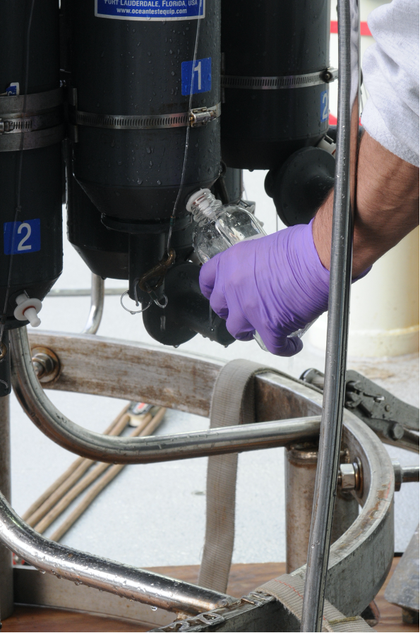
[caption id="attachment_20259" align="alignleft" width="199"] Collecting water samples from the CTD rosette on the Pioneer 8 cruise aboard the R/V Neil Armstrong. ©WHOI.[/caption]
To make these data more easily accessible to the science community, we have developed a common template to provide a full set of discrete water sample data from a cruise. These “Discrete_Sample_Summary” spreadsheets include the details for each Niskin bottle fired on a CTD cast, the CTD instrument rosette data from the time of bottle closure, and the water sample data and quality flags based on World Ocean Circulation Experiment (WOCE) standards.
These CSV files with common data formats can easily be read and manipulated in MATLAB, Python, or other computing programs and languages. Because water analysis data are received at different times from different labs, these spreadsheets are updated as data become available. An accompanying README file contains version history, general notes, and a description of the quality flags. The original spreadsheets from labs, which may contain additional data and methodology, will also be posted.
An example of how to read and use this discrete sample data can be found in this Jupyter notebook. Discrete_Sample_Summary spreadsheets have been posted for the Regional Cabled Array cruises 6-10, the Coastal Endurance Array cruises 1-13, and the Global Irminger Sea Array cruises 1-6. We will continue to work on completing spreadsheets for past cruises as well as cruises going forward.
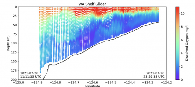
[caption id="attachment_20261" align="aligncenter" width="640"]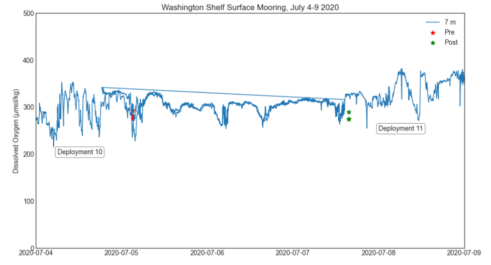 Comparison of dissolved oxygen data on the Washington Shelf Surface Mooring with water sampling data from Endurance Cruise 13. Data from Deployment 10 and Deployment 11 are plotted together, and overlap during 5-7 July.[/caption]
Read More
Comparison of dissolved oxygen data on the Washington Shelf Surface Mooring with water sampling data from Endurance Cruise 13. Data from Deployment 10 and Deployment 11 are plotted together, and overlap during 5-7 July.[/caption]
Read More Putting Data Explorations to Work in Classrooms
 Kathleen Browne, Chair, Geological, Environmental and Marine Sciences Department Rider University[/caption]
It all started with an email blast advertising a workshop offering opportunities to develop new lessons using OOI data. By happenstance, the workshop was right down the street from Kathleen Browne’s office at Rider University in Lawrenceville, New Jersey, making it convenient for her to attend. Sponsored by the National Science Foundation-funded OOI Ocean Data Labs at Rutgers University of New Jersey, the workshop’s focus on “data explorations” meshed nicely with Browne’s long held involvement in advancing science education plans for both higher ed and K-12 teachers. Browne teaches oceanography and served as academic director of Rider’s Science Education and Literacy Center, which works to advance K-12 and college math and science instructors’ use of inquiry-based instruction.
“Since I have been involved in a whole suite of science education lesson plans and I teach oceanography, it seemed like a unique and worthwhile opportunity, “ she explained.
Little did Browne expect that a five-day workshop would lead to her becoming an integral part of the OOI Ocean Data Labs network. She and Gabriela Smalley, a colleague in Rider’s Geological, Environmental and Marine Sciences Department (which Browne chairs) and colleagues from Maine Maritime Academy (Lauren Sahl), University of Kentucky (Rebecca Freeman), Southern Maine Community College (Carol White), and Rutgers (Sage Lichtenwaler) created an OOI data exploration on ocean anoxic events. Browne and Smalley have since also contributed to a new lab manual created by the Ocean Data Labs. Browne created labs in geology, while Smalley contributed labs on primary production and biology.
The pandemic has changed the way Browne is considering classroom instruction. “I’m in the midst of rethinking how I teach labs, particularly given all I’ve learned in these days of remote instruction. It’s hard to teach an oceanography lab remotely when students are clearly looking for something different than what we can do remotely. I imagine, for example, we might use the intro labs in the lab notebook in the beginning of the semester because we are finding that students really need focused guidance on describing patterns in data sets before they can make sense of the results.
“Students struggle with understanding data. But, the need for data analysis is not limited to science. It’s important in politics, health care, and most aspects of life today. We live in a world where an enormous amount of data is presented to us daily. It’s not that everyone needs to process that data, but they do need to at least make sense of the data visualizations that might be offered. It’s my hope that my students can do that so they might be able to recognize when something doesn’t make sense. I’d like my students to be better consumers of data, and skeptics of data so they are not misled.”
Browne‘s interest in the business of students struggling to describe patterns in data has prompted a project to figure out the best instructional ways to help students develop data literacy skills to improve their scientific explanation skills. She teamed with Smalley, Andrea Drewes, a learning scientist in Rider’s Graduate Education, Leadership and Counseling department, and Sage Lichtenwaler, a lead investigator and data wrangler with Ocean Data Labs, on a recently funded NSF project. The project will assess students’ data and science literacy skills — that is understanding the scientific principles involved. The project will use a variety of techniques and resources, including the Ocean Data Lab’s data explorations.
“Our approach will be to help students develop their data literacy skills such as the ability to read a graph correctly and identify and articulate in detail the patterns and trends that they see in the data. With those skills refined we will help to help students learn the science in our courses so they are able to explain something they learned about the data and the science using scientific evidence and reasoning.”
The effectiveness of this approach will be tested in two different classroom settings. One will serve as a control, while the other will integrate tools and instruction to help students work with data visualizations. Ultimately, the team will assess the learning gains in the control and intervention classes. Successful techniques identified will be shared broadly with science instructors, learning scientists, and other educational researchers throughout the nation to improve data literacy among U.S. students.
Browne and her team will begin the formal data collection this fall and expect to report their findings in 2023. “My work with OOI data and the Ocean Data Labs has opened up new avenues of exploration for me, and ultimately will help students’ abilities to use data and science literacy skills to contribute as active citizens to pressing ocean-related issues in the world.”
Read More