
Science Highlights
A Carbon Budget for the Upper Mesopelagic Zone

(Adapted from Stephens et al., 2025)
Upper ocean carbon budgets are difficult to constrain, and those for the mesopelagic zone come with particular challenges. A recent paper by Stephens et al. (2025) took on the challenge of a comprehensive carbon system budget for the upper mesopelagic zone (100-500 m) based on data from the EXport Processes in the Ocean from RemoTe Sensing (EXPORTS) program (Siegel et al., 2016). The 2018 EXPORTS field campaign was conducted at Ocean Station Papa in the Northeast Pacific to take advantage of the relatively modest surface forcing, shallow summer mixed layer, tightly coupled food web, and low mesoscale kinetic energy. Nevertheless, the study found that a steady-state assumption for the carbon system was likely not appropriate.
Measuring organic carbon supply and demand is challenging due to a variety of factors. Supply includes sinking particles, migrating zooplankton and fish, disaggregation, mixing and subduction. Demand comes primarily from bacteria and zooplankton. Measurement methods for each supply and demand term have errors, conversions to rates have uncertainties, and each process being measured may have a unique timescale over which a rate integration makes sense. EXPORTS was notable for increasing the number and variety of measurements available for monitoring the mesopelagic carbon budget. Stephens et al. take advantage of this by combining multiple measurement methods, quantifying errors and applying statistical methods for error analysis.
The authors used observations from multiple sources. Near-surface data came from the PMEL Station Papa surface mooring. Shipboard profile data come from two ships operating during the EXPORTS field campaign as well as the OOI Station Papa cruise in 2018. Additional water column data came from two OOI Slocum gliders, one EXPORTS-operated Seaglider, and BGC Argo floats. The authors examined each carbon supply and demand estimate, calculating an uncertainty and discussing potential limitations (Stephens et al., Table 1). A Monte Carlo approach was used to assess overall uncertainty in supply and demand terms, resulting in the conclusion that supply was insufficient to meet demand (e.g. Fig. 1 below). The error analysis allowed the authors to conclude that the mismatch was not the result of problems in estimating supply or demand, but rather a problem with the assumption that supply and demand would balance within the analysis period. In other words, the system was not in steady state.
This project highlights the complexity of the carbon system in the upper ocean and the broad suite of observational tools necessary to address the carbon budget. The authors make three specific recommendations for improved quantification of the biological carbon pump: including the relevant midwater processes, capturing the range of relevant timescales, and providing redundancy in methodology.
[caption id="attachment_37368" align="alignnone" width="928"]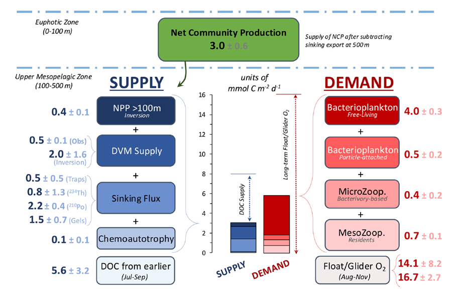 Assessment of the organic carbon budget in the upper mesopelagic zone during EXPORTS. Estimated individual contributions to supply (left) and demand (right) are provided along with error estimates. Terms with multiple measurement methods (far left, far right) were averaged. The center panel shows the cumulative supply and demand relative to a vertical scale in units of mmol C per (m^2 day). From Stephens et al., 2025.[/caption]
___________________
References:
Stephens, B.M., and 20 co-authors, 2025. An upper-mesopelagic-zone carbon budget for the subarctic North Pacific, Biogeosciences, 22, 3301-3328, https://doi.org/10.5194/bg-22-3301-2025.
Siegel, D.A., K.O. Buesseler, M.J. Behrenfeld, C.R. Benitez-Nelson, E. Boss, M.A. Brzezinski, A. Burd, C.A. Carlson, E.A. D’Asaro, S.C. Doney, M.J. Perry, R.H.R. Stanley and D.K. Steinberg, 2016. Prediction of the Export and Fate of Global Ocean Net Primary Production: The EXPORTS Science Plan, Front. Mar. Sci., 3:22, https://doi.org/10.3389/fmars.2016.00022.
Read More
Accounting for Ocean Waves and Current Shear in Wind Stress Parameterization
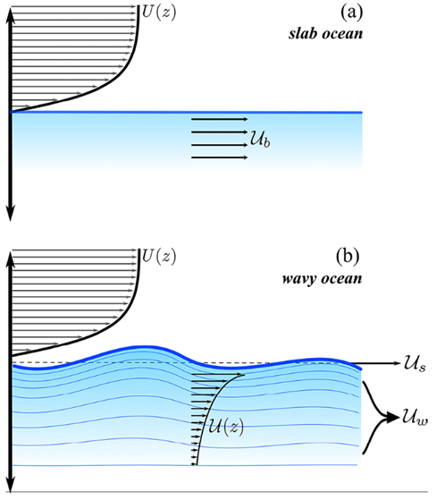
Ortiz-Suslow et al. (2025) use measurements of direct covariance wind stress, directional wave spectra, and current profiles from the OOI Coastal Endurance Array (Ocean Observatories Initiative) offshore of Newport, Oregon (2017–2023) to test a proposed new general framework for the bulk air-sea momentum flux that directly accounts for vertical current shear and surface waves in quantifying the stress at the interface. Their approach partitions the stress at the interface into viscous skin and (wave) form drag components, each applied to their relevant surface advections, which are quantified using the inertial motions within the sub-surface log layer and the modulation of waves by currents predicted by linear theory, respectively.
Their framework does not alter the overall dependence of momentum flux on mean wind forcing, and they found the largest impacts at relatively low wind speeds. Below 3 m s−1, accounting for sub-surface shear reduced form drag variation by 40–50% as compared to a current-agnostic approach. As compared to a shear-free current, i.e., slab ocean, a 35% reduction in form drag variation was found. At low wind forcing, neglecting the currents led to systematically overestimating the form stress by 20 to 50% — an effect that could not be captured by using the slab ocean approach. Their framework builds on the existing understanding of wind-wave-current interaction, yielding a novel formulation that explicitly accounts for the role of current shear and surface waves in air-sea momentum flux. Ortiz-Suslow et al. find their work holds significant implications for air-sea coupled modeling in general conditions.
In using the Oregon Shelf (CE02SHSM) data, Ortiz-Suslow et al. note, “There are several distinct advantages to using these data for this analysis: (1) the range of the dataset goes back seven years with good temporal coverage, (2) there are co-located wind, wave, and current measurements at hourly intervals for in-depth analysis, and (3) the site is exposed to a wide range of wind, wave, and current conditions. Furthermore, by using this dataset, we take advantage of internal quality data control and processing steps that are standardized across the OOI array network.”
[caption id="attachment_37363" align="alignnone" width="488"] Conceptual diagram highlighting the distinction between defining the relative wind velocity over the (a) slab ocean versus the (b) wavy interface. In the presence of near-surface shear, the relative contributions of viscous skin (Us) and wave form (Uw) must be directly accounted when calculating the relative wind at the base of the sheared wind profile (Figure 30, Ortiz-Suslow et al., 2025).[/caption]
___________________
Reference:
Ortiz-Suslow, D.G., N. Laxague, J-V. Björkqvist, M. Curcic, (2025). Accounting for Ocean Waves and Current Shear in Wind Stress Parameterization. Boundary-Layer Meteorology, 191(38), https://doi.org/10.1007/s10546-025-00926-9
Read MoreThe Regional Cabled Array Seen Through the Eyes of Students

One of the OOI’s greatest strengths is its ability to inspire and train the next generation of ocean scientists through immersive, hands-on research at sea and through the analysis and application of large, complex data sets. Students gain authentic, real-world experience in oceanography—working aboard global-class research vessels utilizing advanced robotic vehicles and learning how to communicate their science effectively to broad and diverse audiences. Through the UW VISIONS at-sea experiential learning program more than 200 students have developed these skills while participating in Regional Cabled Array cruises.
Student outcomes are showcased on Interactiveoceans and span an impressive breadth of scientific inquiry. Recent VISIONS’25 projects include short documentaries demystifying hydrophones and distributed acoustic sensing, genetic analyses of deep-sea organisms, and newly developed technologies to probe the metabolomics of life thriving in the extreme environments of hydrothermal vents. These experiences have translated into numerous senior theses with many students presenting their work at professional scientific conferences.
Among the highlights at Ocean Sciences 2026 conference are VISIONS’24–25 student-led presentations that integrated artificial intelligence and computer vision to quantify benthic communities and spatial ecology at Southern Hydrate Ridge. These innovative analyses revealed new connections between biological patterns and methane seep activity, offering fresh insight into the dynamics of this highly active and rapidly changing environment.
[caption id="attachment_37360" align="alignnone" width="445"] RCA Science Highlight: Student Projects and Engagement Products[/caption]
Read More The 2019 marine heatwave at Ocean Station Papa
(Adapted from Kohlman et al., 2024)
Marine Heat Waves (MHW; Hobday et al., 2016) are prolonged periods of extreme ocean sea surface temperature (SST) anomalies. MHWs are typically identified in satellite SST and/or ocean color records; subsurface data and interdisciplinary variables are often lacking. Ocean Station Papa (OSP) provided long-term, interdisciplinary, subsurface data to examine the physical and biochemical characteristics of a MHW in the Northeast Pacific.
MHWs may have multi-faceted causes, as well as impacts on primary production and higher trophic levels. A recent paper by Kohlman et al. (2024) examines the 2019 NE Pacific MHW using gridded satellite SST data and in-situ observations from multiple OSP platforms including the NOAA Pacific Marine Environmental Lab (PMEL) surface mooring, two OOI Flanking Moorings, the Applied Physics Lab (U. Washington) waverider mooring and shipboard samples from OOI and the Department of Fisheries and Oceans, Canada.
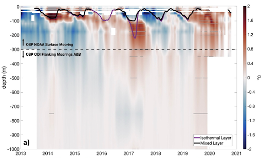
The 2019 MHW was identified in satellite SST data, but the Kohlman et al. study also assessed vertical stratification and the subsurface extent of the temperature signal. The PMEL surface mooring provided temperature and salinity (T/S) down to 300 m. The OOI Flanking Moorings extended the T/S data to 1500 m. The resulting composite time series from 2013-2020 is shown in Fig. 1. Both the extended 2013-2015 MHW and the 2019 MHW are identifiable. Subsurface temperature anomalies during 2013-2014 were strongest above the mixed layer depth (MLD). In the winter and spring of 2017, deeper waters (120–300 m) remained anomalously warm. This anomaly persisted into 2018 due to strong stratification from a fresher surface layer. During the 2019 MHW, anomalously warm waters extended down to 1000 m, whereas the 2013-2015 MHW extended only to about 150 m.
The authors used interdisciplinary data available from Station Papa platforms to assess the drivers and impacts of the 2019 MHW. They found that weaker winds and smaller significant wave height prior to the summer of 2019 created favorable pre-conditioning in the form of an unusually shallow winter MLD. During the MHW, they found that dissolved inorganic carbon and pCO2 decreased, while pH increased. Shipboard samples indicated a decrease in nutrients and an increase in primary productivity. Finally, they speculated that the increased productivity may have had an impact on higher trophic levels – more blue whale calls were recorded in 2019 at Station Papa than normal for Aug-Sep.
This project shows that the characteristics of MHWs are complex. Sustained, multi-disciplinary, subsurface observations are needed to unravel the drivers, pre-conditioning, characteristics, and impacts of these events. Station Papa, among the longest sustained ocean time series sites, is uniquely suited due to the task due to the collaborative observing effort at the site.
[caption id="attachment_37120" align="alignnone" width="512"] Figure 1. Subsurface temperature anomalies at Staton Papa during 2013-2020. Data from the surface to 300 m are from the PMEL surface mooring. Data below 300 m are from the OOI Flanking Moorings. Anomalies are relative to the 1999-2020 Argo climatology. The density-based mixed layer depth (black) and isothermal depth (purple) are overlaid. From Kohlman et al., 2024.[/caption]
___________________
References:
Hobday, A.J., Alexander, L.V., Perkins, S.E., Smale, D.A., Straub, S.C., Oliver, E.C.J., et al. (2016). A hierarchical approach to defining marine heatwaves. Prog. Oceanog., 141(0079–6611), 227–238. https://doi.org/10.1016/j.pocean.2015.12.014.
Kohlman, C., Cronin, M.F., Dziak, R., Mellinger, D.K., Sutton, A., Galbraith, M., et al. (2024). The 2019 marine heatwave at Ocean Station Papa: A multi‐disciplinary assessment of ocean conditions and impacts on marine ecosystems. J. Geophys. Res., 129, e2023JC020167. https://doi.org/10.1029/2023JC020167.
Read MoreSubmarine canyon sediment transport and accumulation during sea level highstand: Interactive seasonal regimes in the head of Astoria Canyon, WA
Lahr et al. (2025) use in-situ hydrodynamic data from a benthic tripod deployment in the head of Astoria Canyon to show that sediment resuspension and transport during summer is driven by internal tides and plume-associated nonlinear internal waves. Observations of shoreward-directed currents and low shear stresses (<0.14 Pa) along with sediment trap data suggest that seasonal loading of the canyon head occurs during summer. Nearby long-term wave data from the OOI Washington Shelf mooring shows that winter storm significant wave height often exceeds 10 m, driving shear stress capable of resuspending all grain sizes present within the canyon head. Swell events are generally concurrent with downwelling flows, providing a mechanism for episodic downcanyon sediment flux. This study indicates that canyon heads can continue to function as sites of sediment winnowing and bottom boundary layer export even with a detached, shelf-depth canyon head.
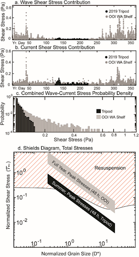
As part of this study, Lahr et al. (2025), used data from the OOI Washington Shelf Surface Mooring located 81 km north of the tripod site in Astoria Canyon. The 2019 benthic tripod deployment by Ogston was done as an ancillary activity on the Endurance 11B cruise aboard R/V Oceanus. The data used were concurrent spectral surface wave and meteorological data near bed current velocity for 2016 (chosen for its complete records). Figure xx shows the benthic tripod stress overlaid with the OOI Washington shelf mooring stress. Over the summer, the benthic tripod stress and OOI estimated stress compare well. Winter stresses (available from OOI mooring only) are much larger than those observed in summer.
[caption id="attachment_37116" align="alignnone" width="277"] Figure 1. Shear stress computed from the Astoria Canyon tripod deployment (black) and the OOI Shelf mooring (gray). Panels a) and b) depict relative stress contributions from waves and currents respectively, c) the distribution of total stresses, and d) maximum shear stresses from summer and winter on a Shields diagram. (Figure 3, Lahr et al., 2025)[/caption]
___________________
Reference:
Lahr, E.J., A.S. Ogston, J.C. Hill, H.E. Glover, and K.J. Rosenberger (2025). Submarine canyon sediment transport and accumulation during sea level highstand: Interactive seasonal regimes in the head of Astoria Canyon, WA. Marine Geology, no. (2025): 107516. https://www.sciencedirect.com/science/article/pii/S0025322725000416.
Read MoreRCA Broadband Provides First Report of Tremor-Like Signals Offshore Cascadia
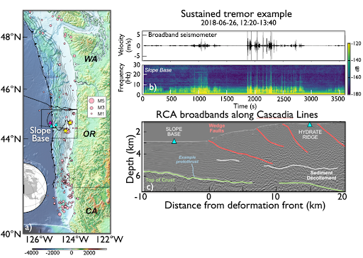
The recent publication “Possible Shallow Tectonic Tremor Signals Near the Deformation Front in Central Cascadia” (Krauss et al., 2025) presents the first report of tectonic tremor-like signals offshore Cascadia. As described by the authors, deep slow-slip events in Cascadia—lasting from hours to weeks—have been documented by land-based stations for decades. These events can accommodate a significant portion of overall plate motion and may serve as precursors to megathrust earthquakes. Over the past two decades, significant tectonic tremor activity (1–10 Hz) has been observed as a feature of slow slip every 10.5–15.5 months beneath Vancouver Island to northern Oregon (Bombardier et al. 2024), with annual slip events equivalent to a magnitude ~6.5 earthquake. These typically occur well inland, at depths of approximately 30–40 km. Contrastingly, it is unknown whether slow-slip events and accompanying tectonic tremor occur at shallow subduction depths in the offshore region.
Krauss et al. (2025) analyzed data collected 2015-2024 from buried ocean-bottom seismometers (OBS) at two sites: Slope Base (2,920 m depth), located 5 km seaward of the deformation front, and Southern Hydrate Ridge (790 m depth), approximately 20 km landward. The analysis incorporated in-situ bottom current data. After applying short- and long-term averaging techniques, the study identified 85,000 signals at Slope Base and 30,055 at Southern Hydrate Ridge, encompassing T-phase events, ship noise, and tectonic tremor-like signals. Notably, tectonic tremor-like signals were observed exclusively at Slope Base.
These signals cannot be attributed to ship traffic or environmental noise. Instead, they are hypothesized to originate from slow slip on one of many nearby tectonic structures: the décollement fault, faults near the subduction zone front and outermost accretionary wedge, faults on the incoming Juan de Fuca Plate, or nearby strike-slip structures such as the Alvin Canyon Fault. However, without additional observations of these signals on multiple stations, it is unclear whether they are tectonic or represent another signal altogether.
Future deployments, such as those planned through the Cascadia Offshore Subduction Zone Observatory (COSZO) will improve our ability to pinpoint the sources of these offshore tremors. The full dataset and results are available on GitHub (https://github.com/zoekrauss/obs_tremor) and archived on Zenodo (https://zenodo.org/records/14532861).
[caption id="attachment_37111" align="alignnone" width="512"] Figure 1. a) Location of the Regional Cabled Array cabled broadband seismometers (OBS’s -cyan triangles) offshore Newport Oregon and an autonomous instrument (purple triangle), earthquakes (pink circles) and along and just offshore the Cascadia Margin. b) sustained tremor-like signals from the broadband at Slope Base. c) Subsurface structure across strike of the margin showing location of Slope Base and Southern Hydrate Ridge OBS’s, accretionary margin faults and demarcation of a boundary interpreted to be a protothrust between the sedimentary column and the incoming Juan de Fuca Plate crust.[/caption]
___________________
References:
Krauss, Z., Wilcock, W.D.S., and Creager, K.C. (2025) Possible shallow tectonic tremor signals near the deformation front in Central Caldera. Seismica, https://seismica.library.mcgill.ca/article/view/1540.
Bombardier, M., Cassidy, J.F., Dosso, S.E., and K. Honn (2024) Spatial distribution of tremor episodes from long-term monitoring in the northern Cascadia Subduction Zone. Journal of Geophysical Research, https://doi.org/10.1029/2024JB029159.
Read MoreSAR Imagery Detects Atmospheric Stratification
(Adapted from Stopa et al., 2024)
There is interest in using satellite-based Synthetic Aperture Radar (SAR) imagery to assess phenomena related to atmospheric boundary layer stratification over the ocean. Obtaining such information with high spatial and temporal resolution would advance boundary layer research and would be beneficial to the development of offshore wind energy. However, monitoring marine boundary layer structure remotely is a challenge. A recent paper by Stopa et al. (2024) shows that it is possible to utilize SAR imagery, in conjunction with in-situ meteorology, to characterize boundary layer stratification.
The Central Surface Mooring (CNSM) of the OOI Pioneer New England Shelf Array is located near a region of offshore wind development where SAR imagery is also available. The authors use wind speed, air temperature, and sea surface temperature from the CNSM buoy to estimate the bulk Richardson number (Ri), a measure of marine atmospheric boundary layer stability. OOI quality control flags were used to identify good data, and suspect data were replaced with data from redundant sensors. CNSM data from 2014 – 2021 were used in the analysis.
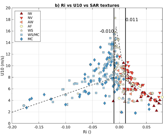
SAR data are commonly used to provide wind speed estimates, but the images also contain rich information about coherent structures in the atmosphere, and those structures correspond to boundary layer stratification regimes (Stopa et al., 2022). The Stopa et al., (2024) study used European Space Agency Sentinel-1 C-band SAR wave mode (S1 WV) imagery spanning the region of the NES Pioneer Array. SAR Images in 20 x 20 km regions were visually examined and classified based on observed “signatures” of atmospheric phenomena. Of particular interest for this study were signatures indicative of waves, rolls/streaks and convection (Table 1).
The relationship of SAR image classes to wind speed and atmospheric stability was examined by plotting the classified data set vs Ri and U10 (Figure 1). U10 shows a change in slope near neutral stratification (Ri = 0) with indications of a Ri-U10 relationship at higher and lower Ri. Of interest is the appearance of Ri boundaries denoting transitions between unstable (Ri < -0.01), neutral, and stable (Ri > 0.01) regimes. Rolls, streaks and convection dominate the unstable regime, while waves dominate the stable regime. In other words, classification of the SAR images provides information about atmospheric stratification.
This project shows the power of combining remote sensing with long-term, in-situ meteorological measurements to gain insights that neither could provide alone. The authors note that when satellite data are available, the SAR-based determination of boundary layer structure can be used over broad areas and long times, and is more efficient than direct measurements such as buoy-based LIDAR.
Table 1: Atmospheric signatures in SAR imagery
| Class | Phenomena |
| NV | Lack of rolls or cells |
| AW | Atmospheric gravity waves |
| IW | Oceanic internal gravity waves |
| WS | Rolls or wind streaks |
| MC | Microscale convection |
| WS/MC | Combined WS/MC |
Figure 1. SAR image classes shown as different symbols) vs. Richardson number (Ri) and ten meter wind speed (U10). Note the regime transitions near Ri = -0.01 and +0.01. From Stopa et al., 2024.[/caption]
___________________
References:
Stopa, J.E., C. Wang, D. Vandemark, R.C. Foster, A. Mouche, and B. Chapron, (2022). Automated Global Classification of Surface Layer Stratification Using High-Resolution Sea Surface Roughness Measurements by Satellite Synthetic Aperture Radar,” Geophysical Research Letters 49(12), e2022GL098686.
Stopa, J.E., D. Vandemark, R. Foster, M. Emond, A. Mouche, and B. Chapron (2024). Characterizing the Atmospheric Boundary Layer for Offshore Wind Energy Using Synthetic Aperture Radar Imagery. Wind Energy, 27:1340–1352, https://doi.org/10.1002/we.2933.
Read MoreGap-Filled Dissolved Oxygen Data from the Ocean Observatories Initiative Endurance Array Inshore Moorings

Brandy Cervantes contributed the dataset described below to Zenodo. This dataset now appears in the OOI Community Datasets under the OOI home page.
The National Science Foundation Ocean Observatories Initiative (OOI) collects continuous in-situ measurements of dissolved oxygen (DO) on the Endurance Array moorings in the inner shelf region of the Oregon and Washington coasts. Aanderaa Optode 4831 oxygen sensors were deployed at 7 meters depth on the near surface instrument frame (NSIF) and on the collocated coastal surface piercing profiler (CSPP) moorings. The sensors suffer from calibration drift due to biofouling, which can cause a dramatic increase in DO during daylight hours and corresponding decrease at night compared to the conditions in the water column. This enhanced diel signal, when present, is much more pronounced on fixed-depth sensors and usually begins to occur 1-2 months after a mooring is deployed. After this biofouling issue was identified, OOI began deploying UV lamps adjacent to the oxygen sensor in spring 2018, after which there was substantial improvement in DO data quality. Each file in this dataset contains the measured near surface DO and the corrected near surface DO at the Oregon and Washington inner shelf surface moorings (ISSM) with gaps from periods of biofouling replaced with the DO measured by the CSPP.
___________________
References:
Cervantes, B. (2025). Gap-Filled Dissolved Oxygen Data from the Ocean Observatories Initiative Endurance Array Inshore Moorings [Data set]. Zenodo. https://doi.org/10.5281/zenodo.15742508
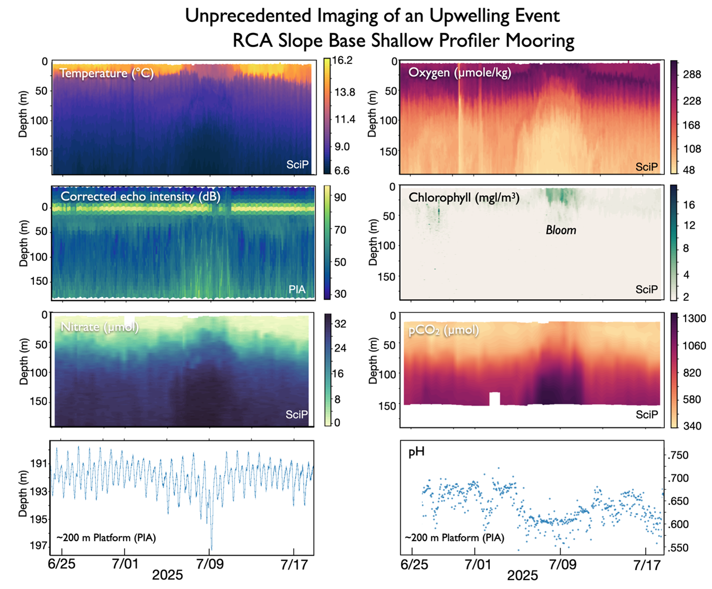
Read MoreUnprecedented Imaging of an Upwelling Event: RCA Slope Base Shallow Profiler Mooring
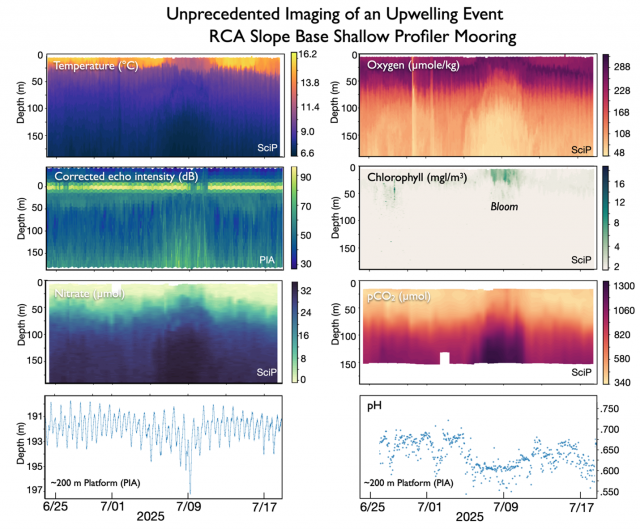
Co-registered instruments on the Slope Base Shallow Profiler Mooring, located 108 km offshore Newport, Oregon, yield unprecedented high resolution imagery of a possible short-lived upwelling event and resultant bloom, ~July 5-13, 2025. The above plots from live streaming data from sensors on the stationary platform interface assembly (PIA) located at ~ 200 m water depth (150 kHz ADCP, CTD-O2, and pH), and on an instrumented winched science pod (SciP)(CTD-O2, nitrate, pCO2, 3 wavelength fluorometer), which traverses 9 times a day from ~ 200 m to ~ 5 m beneath the ocean’s surface, highlight the arrival of cold, nutrient-rich water to the surface layers, coinciding with elevated chlorophyll-A concentrations and increased echo intensity in the ADCP data, as well as increased pCO2 and decreased dissolved oxygen concentrations at depth. These trends are coincident with a decrease in temperature, conductivity, dissolved oxygen concentrations, and pH on the PIA. In contrast to the SciP chlorophyll profile, which indicate a bloom in the surface waters above 50 meters, the PIA chlorophyll-A concentrations show no active blooms in the deeper waters. Interestingly, this event coincides with an increase of sea water pressure as measured at the 200 platform, indicating possible current forcing from the NE (and eddy?) acting to “blow down” the platform by ~ 6 m. Several other blow down events have occurred at the Slope Base and Oregon Offshore sites, the largest of which in the summer of 2019 blew the Slope Base platform nearly 50 m deeper and ~350 m to the west.
Salinification of the Cold Pool on the New England Shelf

(Adapted from Taenzer et al., 2025)
The continental shelf within the Mid-Atlantic Bight is cooled and mixed vertically in the winter. This relatively cold, fresh water is trapped below the seasonally-warming surface layer, retaining its properties as a subsurface “cold pool” throughout most of the spring and summer. The cold pool is important for regional ecosystems, serving as a cold-water habitat and a nutrient reservoir for the continental shelf. It is known that the cold pool warms and shrinks in volume as a result of advective fluxes and heat exchange with surrounding waters. A recent paper by Taenzer et al. (2025) shows for the first time that the cold pool is also subject to salt fluxes and increases significantly in salinity from April to October.
The Pioneer New England Shelf (NES) inshore moorings (ISSM and PMUI) are positioned shoreward of the shelfbreak front and sample conditions on the outer continental shelf where the cold pool can be identified. The authors extracted data from these two moorings from a quality-controlled data set containing timeseries of hydrographic data (temperature, salinity and pressure) from all of the Pioneer NES moorings on a uniform space-time grid, covering the timeframe from January 2015 through May 2022 (Taenzer et al., 2023). The cold pool study used data from 2 m depth, 7 m depth, and 2 m above the bottom on ISSM and from roughly 28 m to 67 m depth on PMUI.
Seven years of data from the Pioneer ISSM and PMUI moorings were used to create a composite annual cycle, which showed that subsurface salinity on the outer shelf consistently increases in the spring and summer. Evaluating the 67 m depth salinity record, and restricting the time period to when the moorings are in the cold pool, resulted in a salinification estimate of 0.18 PSU/month, or ~1 PSU over the six month period (Figure 34a). It was shown that this salinity change could not be explained by a seasonal change in the frontal position.
Isolating the corresponding cold pool region within the New England Shelf and Slope (NESS) model (Chen and He, 2010), and computing a similar multi-year mean, showed a salinification trend nearly identical to that from the observations (Figure 34b). Using the model, it was possible to define a three-dimensional cold pool volume and estimate terms in the cold pool salinity budget. It was found that cross-frontal fluxes transport salt from offshore to the cold pool at a relatively steady rate throughout the year, and that along-shelf advection contributes little to the salinification process. It was argued that the cold pool exhibits two regimes that result in the seasonal salinification: During the winter, vertical mixing is strong, and the cold pool gets replenished with fresh water from the surface layer, which tends to balance the cross-shelf salt flux. During the spring and summer, surface stratification increases, vertical mixing is inhibited, the cold pool is effectively isolated from surface mixing, and the cross-shelf salt flux results in cold pool salinification.
This project shows the importance of long-duration observations in key locations to isolate phenomena that would not be identifiable from a short-term process study. It is notable that the authors undertook a significant quality control effort and created a merged, depth-time gridded data set that was made publicly available. By combining the observations with a high-resolution regional model, the authors were able to examine the cold pool salinity budget and attribute the observed signals to ocean processes.
[caption id="attachment_36391" align="alignnone" width="402"] Figure 34: The seven-year mean annual cycle of continental shelf cold pool salinity from a) Pioneer Array PMUI salinity at 67m depth, b) NESS model salinity for all waters below 10◦C along 70.875 W. The shaded envelope depicts one standard deviation of interannual variability. The salinification trend is from a linear fit during the stratified season (April-October). From Taenzer et al., 2025.[/caption]
___________________
References:
Chen, K., & He, R. (2010). Numerical investigation of the Middle Atlantic Bight Shelfbreak Frontal circulation using a high-resolution ocean hindcast model. J. Physical Oceanog., 40 (5), 949 – 964. doi:10.1175/2009JPO4262.1
Taenzer, L.L., G.G. Gawarkiewicz and A.J. Plueddemann, (2023). Gridded hydrography and bulk air-sea interactions observed by the Ocean Observatory Initiative (OOI) Coastal Pioneer New England Shelf Mooring Array (2015-2022) [data set], Woods Hole Oceanographic Inst., Open Access server, https://doi.org/10.26025/1912/66379.
Taenzer, L.L., K. Chen, A.J. Plueddemann and G.G. Gawarkiewicz, (2025). Seasonal salinification of the US Northeast Continental Shelf cold cool driven by imbalance between cross-shelf fluxes and vertical mixing. J. Geophys. Res., accepted.
Read More