
Science Highlights
Subsurface Temperature Anomalies off Central Oregon during 2014–2021

Brandy T. Cervantes, Melanie R. Fewings, and Craig M. Risien
Cervantes et al. (2024) use water temperature observations from a stationary oceanographic platform located in 80 m water depth off Newport, Oregon to calculate variations from the long term mean temperature at the surface, near surface, and bottom from 1999 to 2021. This site, known as NH-10, was occupied since 1999 successively by an Oregon State University National Oceanographic Partnership Program (OSU NOPP), GLOBEC Long Term Observation Program, Oregon Coastal Ocean Observing System (OrCOOS), NANOOS/CMOP. Since 2015 it has been occupied by the NSF OOI Coastal Endurance Oregon Shelf mooring (CE02SHSM). The temperature observations from these different programs that have not previously been combined into one long time series. Of particular interest are the details of the marine heatwave (MHW) periods of 2014–2016 and 2019– 2020, which had widespread impacts on marine ecosystems. Strong deviations from the mean water temperature observed near the ocean bottom during late 2016 are the largest sustained warm anomalies in the time series. The 2019–2020 period shows warm anomalies in the summer and fall that are only observed near the surface.
They also analyze the local winds during years with and without MHWs and find that spring/summer upwelling favorable, or northerly winds, which are important for bringing cold, nutrient rich water to the surface in coastal regions, interrupt MHW events and can lessen extreme heating during MHWs in coastal waters as illustrated in Figure 33.
The three periods detailed in Figure 33 show warmer daily surface temperatures during the MHW years than the non‐MHW years and several days during 2014–2016 with surface and bottom anomalies greater than 4°C and during 2014–2016 and 2019–2020 with surface anomalies greater than 4°C (Figure 12a). During upwelling favorable winds (negative wind stress), the three periods follow similar patterns with colder surface temperatures typically associated with higher wind stress magnitudes. During downwelling‐favorable winds (positive wind stress), 2014–2016 is substantially warmer at the surface than the other periods at all wind stress values.
[caption id="attachment_36388" align="alignnone" width="526"] Figure 33: 8‐Day low‐pass filtered surface temperature at NH‐10/CE02SHSM for (a) 1999–2000, (d) 2014–2015, and (g) 2019–2020; 8‐day low‐pass filtered along‐shelf surface velocity for (b) 1999–2000, (e) 2014–2015, and (h) 2019–2020; and NDBC 46050 wind stress vectors (thin light lines) and along‐shelf 8‐day wind stress (thick lines) (c) 1999–2000, (f) 2014–2015, and (i) 2019–2020. Events identified as surface marine heatwaves are shaded in gray. The thick black line in panels (a–b), (d–e), and (g–h) is the climatological mean computed over the full NH‐10 time series (Figure 33c), repeated twice, and the thin black lines are the 90th and tenth percentiles.[/caption]
___________________
References:
Cervantes, B. T., Fewings, M. R., & Risien, C. M. (2024). Subsurface temperature anomalies off central Oregon during 2014–2021. Journal of Geophysical Research: Oceans, 129, e2023JC020565. https://doi.org/10.1029/2023JC020565
Read MoreSoundscapes Spanning the Oregon Margin and 300 Miles Offshore

 Figure 32: An example of a daily spectrogram generated by the RCA Data Team spectrogram viewer. A Humpback whale song is visible throughout the day at ~40-1000 Hz. A chorus of Fin Whale vocalizations is visible at 20-40 Hz. A weather event is visible at 0100, and a ship passage at 2200.[/caption]
The Regional Cabled Array (RCA) operates six broadband hydrophones that continuously capture soundscapes across the Cascadia Margin (Oregon Shelf and Oregon Offshore – seafloor), near the toe of the margin (Slope Base -seafloor and 200 m water depth) and 300 miles offshore at Axial Seamount (Axial Base – seafloor and 200 m water depth). The hydrophones, operational since 2014, capture signals from 10-64,000 Hz, including vessel traffic, marine mammal vocalization, wind, surf, and seismic events. The RCA broadband acoustic archive currently contains forty years (350,000 hours) of acoustic data in miniSeed format.
The RCA Data Team has developed a pipeline that can summarize and visualize a year of hydrophone data in 30 minutes. The spectrograms output (see Figure 32) by this pipeline are now easily accessible through an interactive viewer on the RCA’s Data Dashboard. The spectrogram viewer will make OOI-RCA broadband hydrophone data more searchable and accessible to data users and strengthen QA/QC of RCA acoustic data. Any day of hydrophone data, since 2014, will be viewable in minute/hybrid-millidecade resolution. The pipeline also enables users to convert RCA acoustic data to audio format (FLAC or WAV) in bulk. The spectrogram viewer was developed with input and guidance from the Ocean Data Lab at University of Washington and the Monterey Bay Aquarium Research Institute Soundscape team. It utilizes open source acoustic software tools – ooipy, pypam, and mbari-pbp.
Read MoreIrminger Sea Convection and the roles of Atmospheric Forcing and Stratification

The high-latitude North Atlantic, is a region where seasonal convection results in deep water formation, a process critical to the Atlantic Meridional Overturning Circulation (AMOC). Surface cooling by cold air and strong winds in the Irminger Sea transforms the surface water and drives deep convection in winter. Prior studies have shown that AMOC strength is linked to the extent of water mass transformation in the Irminger Sea and Iceland Basin. A study by de Jong et al. (2025) used a 19-year time series with weekly resolution compiled from moorings and Argo floats to evaluate the year-to-year variability of deep convection and its relationship to atmospheric forcing versus water column stratification.
A time series of surface forcing for the 19-year analysis period (2002-2020) was obtained from the European Center for Medium-range Weather Forecasting (ECMWF) ERA-5 global atmospheric reanalysis. Hydrographic data from the near-surface to 2500 m was collected from three sources: the NIOZ Long-term Ocean Circulation Observations (LOCO) mooring, the GEOMAR Central Irminger Sea (CIS) mooring, and the OOI Hybrid Profiler Mooring (HYPM). Surface temperature and salinity from Argo, ERA-5, and the OOI surface mooring, along with nearby Argo profiles, were used to provide data at the surface and in the upper water column. The records were merged with 25 m vertical resolution and one week time resolution. Mixed layer depth was determined from the hydrographic profiles using a published algorithm with further quality control using multiple criteria.
The time series of potential vorticity (PV) and mixed layer depth (MLD; Fig. 1d), highlights the significant interannual variability. Some years (e.g. 2002-2003) show relatively shallow winter MLD and little evidence of sustained low PV (which would indicate deep mixing) between years. Other years (e.g. 2015-2016) show strong convection, deep MLD, and sustained low PV. While the change in stratification due to warming and freshening related to climate change is expected to weaken convection future convection, analysis showed that in this record there was a strong correlation between the annual maximum MLD and the total accumulated winter heat loss. The correlation between maximum summer stratification and maximum MLD the following winter was not significant. Thus, among other findings, the authors concluded that during the period analyzed atmospheric forcing is three times more important than pre-existing stratification in determining the maximum winter mixed layer depth in the Irminger Sea.
The processed and edited temperature and salinity profiles from the OOI Irminger Sea HYPM from September 2014 to May 2020 are described by Le Bas (2023). The processed data are publicly available from the NOAA National Centers for Environmental Information (NCEI) and referenced with a DOI. The NCEI record includes information about data quality control, validation and drift correction, gridding method, and algorithms for computation of data products.
This project shows the potential for long-duration OOI moored profiler records to be combined with other data sources to provide unique insights into interannual variability of mixing and deep convection in the Irminger Sea. It is notable that the authors undertook a significant data quality control effort and took advantage of the OOI shipboard validation CTD casts (along with non-OOI CTD data sources) in their processing.
[caption id="attachment_35691" align="alignnone" width="624"] Figure 29: Time series of the combined LOCO, CIS, OOI and Argo record from 2002-2020. a) temperature, b) salinity, c) potential density and d) potential vorticity with mixed layer depth overlaid (black dots). From de Jong et al., 2025.[/caption]
___________________
References:
De Jong, M.F, K.E Fogaren, L. LeBras, L. McRaven and H. Palevsky, (2025). Atmospheric forcing dominates the interannual variability of convection strength in the Irminger Sea. J. Geophys. Res., 130, e2023JC020799. https://doi.org/10.1029/2023JC020799.
Le Bras, I. (2023). Water temperature and salinity profiles from the Ocean Observatories Initiative Global Irminger Sea Array Apex profiler mooring from September 2014 to May 2020 (NCEI Accession 0285241). NOAA National Centers for Environmental Information. Dataset. https://doi.org/10.25921/wzvr-fk49.
Read MoreBloom Compression Alongside Marine Heatwaves Contemporary with the Oregon Upwelling Season

Black et al. (2024) examine the impacts of marine heatwave (MHW) events on upwelling-driven blooms off the Oregon coast. They combine OOI data from Endurance moorings off Oregon with satellite data and indices of upwelling and MHW presence to determine how MHW’s impact these blooms. Their work focuses on MHWs and coincident events that occurred off Oregon during the summers of 2015–2023. They found the presence of MHW’s limited the offshore extent of phytoplankton blooms. In late summer 2015 and 2019, both documented MHW years, coastal phytoplankton biomass extended on average 6 and 9 km offshore of the shelf break along the Newport Hydrographic Line, respectively. During years not influenced by anomalous warming, coastal biomass extended over 34 km offshore of the shelf break. Reduced biomass also occurs with reduced upwelling transport and nutrient flux during these anomalous warm periods. However, the enhanced front associated with a MHW aids in the compression of phytoplankton closer to shore. Over shorter events, heatwaves propagating far inshore also coincide with reduced chlorophyll a and sea-surface density at select cross-shelf locations, further supporting a physical displacement mechanism. Paired with the physiological impacts on communities, heatwave-reinforced physical confinement of blooms over the inner-shelf may have a measurable effect on the gravitational flux and alongshore transport of particulate organic carbon. Black is a PhD student at Oregon State University and notes that all data used in the paper, including of course OOI data, are open source. They provide details regarding data access methods and intermediate processing steps along with code modules to reproduce the work at https://github.com/IanTBlack/oregon-shelf-mhw.
Black et al. focus much of their analysis on the Oregon Offshore mooring, CE04 (Fig. x). Here they show individual warm events aligned with periods where Chl a was much lower than the time-series average and the climatological mean. The analysis period for 2019 had the lowest average Chl a across all years. From the CE04-derived Chl a climatology, they observed an occurrence of a regular spring bloom (April) and a summer bloom (September). The peak of the summer bloom appears contemporary with the warmest time of year at CE04, and years 2019 and 2023 were the only years that experienced MHWs during this same period. The summer blooms of 2019 and 2023 at CE04 were also noticeably suppressed and difficult to differentiate from surrounding Chl a values.
[caption id="attachment_35688" align="alignnone" width="624"] Figure 28: Ocean Observatories Initiative (OOI) CE04, Coastal Upwelling Transport Index (CUTI), and Biologically Effective Upwelling Transport Index (BEUTI) time series between 2015 and 2023. Daily mean values are in light blue. Red vertical spans indicate potential marine heatwave (MHW) events and gray vertical spans indicate the time between the spring and fall transition dates. A centered 11-d rolling mean was applied to smooth the data (black).[/caption]
___________________
Reference:
I Black, IT, Kavanaugh, MT, Reimers, CE. “Bloom compression alongside marine heatwaves contemporary with the Oregon upwelling season.” Limnology and Oceanography, no. (2024): First published: 16 December 2024, https://doi.org/10.1002/lno.12757
Read MoreBringing Computer VISION into the Classroom Utilizing RCA Imagery and the OOI Jupyter Hub

There is a rapidly growing demand in Earth system science for workforce expertise in machine learning. To increase marine science students understanding of, and ability to use, artificial intelligence tools, Dr. Katie Bigham and School of Oceanography undergraduate student Atticus Carter are teaching an undergraduate class focused on applying “computer vision” (processing imagery with the computer) to marine science problems. The Computer Vision Across Marine Sciences prototype course for UW undergraduates in the Ocean Technology program includes the development of a Jupyter Binder (a notebook collecting multiple Jupyter Notebooks). Currently, an enormous amount of time is required to manually process imagery collected in marine environments, resulting in a major bottleneck for all research utilizing marine imagery. In this course, students gain an understanding of computer vision capabilities, model training and evaluation, and research applications. The course utilizes real-world datasets from the OOI Regional Cabled Array (RCA), including imagery from remotely operated vehicles utilized on RCA cruises and fixed camera imagery on the array, and from other systems, exposing students to diverse marine habitats. For their final projects, students will develop bespoke models utilizing datasets of their choosing, including RCA imagery. Students can employ the OOI Jupyter Hub for additional computational power, facilitating easy access to imagery and necessary resources. In collaboration with a faculty member in the UW School of Education quantitative data are collected on student learning and feedback for course improvement. The open-access course text is actively under development and is accessible at OceanCV.org. The team aims to improve the materials based on student feedback. Carter will present findings and learnings from the first version of the class at ASLO 2025 Aquatic Sciences Meeting in the Building Data Literacy Skills in the Next Generation of Aquatic Scientists session hosted by OOI Data Labs.
[caption id="attachment_35685" align="alignnone" width="640"] Figure 27: Introductory page for Computer Vision Across Marine Sciences Jupyter Binder and example of artificial intelligence-based predictions of animals in imagery collected by the Regional Cabled Array digital still camera at Southern Hydrate Ridge. This work is supported by an NSF OCE Postdoctoral Research Fellowship to Dr. K. Bigham, University of Washington.[/caption]
Read More Irminger Sea Carbon Cycle
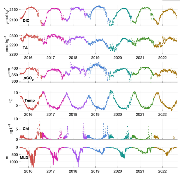
The high-latitude North Atlantic, a region with high phytoplankton production in the spring and deep convection in the winter, is of particular importance for the global carbon cycle. The vertical transport of carbon from near the surface into the deep ocean, by combination of biological and physical processes, is known as the biological carbon pump. The carbon pump is particularly active in the Irminger Sea, yet the carbon budget, and its seasonal and interannual variability, are poorly known. A study by Yoder et al. (2024) used carbon system data from multiple observational assets (moorings and CTD casts) of the OOI Irminger Sea Array to assess net community production in the mixed layer and the implications for the biological pump in this region.
Data analysis was challenging, because it involved working with multiple instrument types, gappy records, calibration offsets, and other idiosyncrasies. In addition, data from multiple instruments and observing platforms needed to be combined to produce continuous records. The primary sensors utilized were pH and pCO2. These are difficult sensors to work with, to the extent that a community workshop was convened to develop a “users guide” to best practices for analysis (Palevsky et al., 2023). Yoder et al. were able to quality control, cross-calibrate, and merge data from the OOI surface mooring, flanking moorings, gliders and shipboard CTD casts (Fogaren and Palevsky 2023; Palevsky et al. 2023) to create the first multi‐year time series of the inorganic carbon system for the Irminger Sea mixed layer. This remarkable data set, based on instruments with sample rates of 1-2 hours, provides a seven-year record with near-daily resolution (Figure 28).
The time series results (Figure 3) showed that carbon system variables (dissolved inorganic carbon (DIC), total alkalinity (TA), and partial pressure of CO2 (pCO2)) co-vary through the annual cycle, with minimums in late summer at the end of the productive season and maximums in winter. The summer draw-down of pCO2 indicates that biophysical effects, rather than temperature, are the primary drivers of pCO2 variability. The influence of vertical mixing and primary productivity can be clearly seen in DIC and TA. In the subpolar North Atlantic, shoaling of the mixed layer in spring is generally associated with spring phytoplankton blooms, as indicated by increasing chlorophyll (Chl) concentration. Interestingly, it is found that highest integrated rates of DIC removal from the mixed layer via photosynthesis take place prior to mixed layer shoaling.
After a thorough analysis that included mixed layer budgets of DIC and TA, followed by assessment of gas exchange, physical transport, and the hydrologic cycle, the authors conclude that strong biological drawdown is the primary removal mechanism of inorganic carbon from the mixed layer. Furthermore, they point out the importance of interannual variability in both the drivers of and resulting magnitude of surface carbon cycling. This is primarily due to variability in net community production. Acknowledging the challenges taken on by OOI to maintain an array in the Irminger Sea, the authors note that “collecting observational data is both costly and challenging, however if only 1 year of data is collected or multiple years are averaged together, [carbon system dynamics] … will be misrepresented.”
This project shows the potential for OOI data, with appropriate processing and analysis, to provide unique insights into the ocean carbon system. It is notable that the authors made a substantial effort to calibrate and combine data from multiple instruments and moorings, and to take advantage of ancillary data (e.g. gliders, OOI CTD casts, and non-OOI CTD casts) in their processing. Enabling this type of analysis was a goal in the design of the multi-platform OOI Arrays and shipboard validation protocols.
[caption id="attachment_34983" align="alignnone" width="623"] Time series of dissolved inorganic carbon (DIC), total alkalinity (TA), partial pressure of CO2 (pCO2) temperature, chlorophyll-a (Chl), and mixed layer depth (MLD) in the Irminger Sea mixed layer from 2015-2022. Colors identify annual cycles. From Yoder et al., 2024.[/caption]
___________________
References:
- Fogaren, K. E., Palevsky, H. I. (2023) Bottle-calibrated dissolved oxygen profiles from yearly turn-around cruises for the Ocean Observations Initiative (OOI) Irminger Sea Array 2014 – 2022. Biological and Chemical Oceanography Data Management Office (BCO-DMO). Version Date 2023-07-19 doi:10.26008/1912/bco-dmo.904721.1
- Palevsky, H.I., S. Clayton and 23 co-authors, (2023).OOI Biogeochemical Sensor Data: Best Practices & User Guide Global Ocean Observing System, 1(1.1), 1–135. https://doi.org/10.25607/OBP-1865.2
- Palevsky, H. I., Fogaren, K. E., Nicholson, D. P., Yoder, M. (2023) Supplementary discrete sample measurements of dissolved oxygen, dissolved inorganic carbon, and total alkalinity from Ocean Observatories Initiative (OOI) cruises to the Irminger Sea Array 2018-2019. Biological and Chemical Oceanography Data Management Office (BCO-DMO). Version Date 2023-07-19 doi:10.26008/1912/bco-dmo.904722.1
- Yoder, M. F., Palevsky, H. I., & Fogaren, K. E. (2024). Net community production and inorganic carbon cycling in the central Irminger Sea. J. Geophys. Res., 129, e2024JC021027. https://doi.org/10.1029/2024JC021027
Impact of Ocean Model Resolution on Temperature Inversions in the Northeast Pacific Ocean
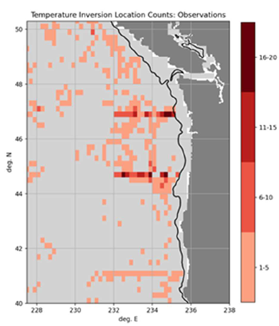
Temperature inversions are a local vertical minimum in temperature located at a shallower depth than a local maximum. In the Northeast Pacific, several water masses and multiple mechanisms for transforming or advecting ocean temperature (cold air events, upwelling, river discharge, cross-shelf eddy transport) create favorable conditions for temperature inversions. Modeling these temperature inversions is challenging. Osborne et al. (2023) analyze observations from 2020 and 2021 to characterize inversions in the Northeast Pacific. The data for these observations come largely from OOI Endurance Array gliders accessed through the GTS database. They compare the observed inversions to model results from the U.S. Navy’s Global Ocean Forecast System version 3.1 (GOFS 3.1) and two instances of the Navy Coastal Ocean Model. Temperature inversions are observed to be present in about 45% of profiles with temperature minimums between 50 – 150 m, temperature maximums between 75 – 175 m, and inversion thickness almost entirely less than 40 m. Modeled temperature inversions are present in only about 5% of model-observations comparisons, with weaker, shallower minimums. This is attributed to two primary causes: coarse model resolution at the inversion depth and the assimilation process which low-pass filters temperature, making inversions weaker. Osborn et al. identify additional work to test the impact of vertical grids on improving model performance.
[caption id="attachment_34977" align="alignnone" width="392"] Maps of inversion counts for observed profiles collected during 2020-2021 and analyzed in this work. Profiles have been filtered to be offshore of the 200 m isobath and to only one profile per collection platform per day (e.g., one profile per glider per day). Black line near the coast marks the 200 m isobath. Light gray indicates no profiles collected during the study period.[/caption]
___________________
References:
J. Osborne V, C. M. Amos and G. A. Jacobs, “Impact of Ocean Model Resolution on Temperature Inversions in the Northeast Pacific Ocean,” OCEANS 2023 – MTS/IEEE U.S. Gulf Coast, Biloxi, MS, USA, 2023, pp. 1-8, doi: 10.23919/OCEANS52994. 2023.10337390.
Read MoreNew Hints When Axial Might Erupt: Precursor Events Detected Through Machine Learning
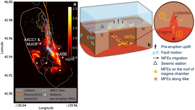
A recent paper by Wang et al., “Volcanic precursor revealed by machine learning offers new eruption forecasting capability” [1] describes the characterization of time-dependent spectral features of earthquakes at Axial Seamount prior to the 2015 using unsupervised machine learning (this method applies algorithms to analyze data without humans in the loop). A major finding from this work is the identification of a distinct burst of mixed-frequency earthquake (MEF) signals that rapidly increased 15 hours prior to the start of the eruption, peaked one hour before lavas reached the seafloor, and earthquakes at Axial Seamount prior to the 2015 using unsupervised machine learning (this method applies algorithms to analyze data without humans in the loop). A major finding from this work is the identification of a distinct burst of mixed-frequency earthquake (MEF) signals that rapidly increased 15 hours prior to the start of the eruption, peaked one hour before lavas reached the seafloor, and migrated along pre-existing faults. The earthquakes are thought to reflect brittle failure driven by magma migration and/or degassing of volatiles. The source mantle beneath Axial Seamount contains extremely high CO2 concentrations leading to high concentrations in the melts [3,4]. MEFs were detected for months prior to the eruption, which could result from volatile release associated with inflation of the sills that feed Axial [5]. Importantly, the identification of these signals may help forecasting of the upcoming Axial eruption and may also be applied to other active volcanoes.
The authors utilized a wealth of geophysical data from the past decade to present an integrated view of Axial (Figure 1) including a subset of earthquake data 4 months prior to the eruption (67,767 out of their >240,000 earthquake catalogue from the RCA seismic array [2]), coupled with bottom pressure from BOTPT instruments at the Central Caldera and Eastern Caldera sites, and 3D modeling.
[caption id="attachment_34973" align="alignnone" width="640"]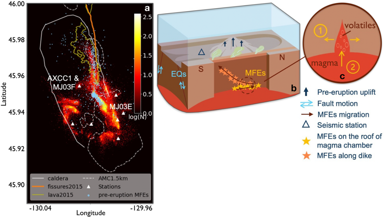 After Wang et al., 2024 [1] Figures 1 and 4: a) Heatmap of earthquake density at Axial Seamount from Nov 2014 to Dec 2021 [2]. Image highlights mixed‐frequency earthquakes (MFEs – light blue dots) one day before the eruption, the caldera rim (white solid line), the 1.5 km depth contour of the Axial magma chamber (AMC)(dashed white line), eruptive fissures (orange lines), lava flows of the 2015 eruption (yellow lines), the location of the RCA short-period seismometer array (white triangles),broadband seismometer AXCC1 and bottom pressure tilt instruments (MJ03E and MJ03F. Heatmap shows the number of earthquakes in each 25 m × 25 m bins. b) Cartoon summarizing observations. Tidally‐driven earthquakes occur on caldera ring faults, while the MFEs track movement of volatiles and magma prior to the eruption. c) possible mechanisms of the MFEs. ① and ② correspond to crack opening and volatile/magma influx processes.[/caption]___________________
References:
[1] Wang, K., F. Waldhouser, M. Tolstoy, D. Schaff, T. Sawi, W.S.D. Wilcock, and Y.J. Tan (2024) Volcanic precursor revealed by machine learning offers new eruption forecasting capability. Geophyiscal Research Letters, 51 (19) https://doi.org/10.1029/2024GL108631.
[2] Wang, K., F. Waldhouser, D.P. Schaff, M. Tolstoy, W.S.D. Wilcock, and Y.J. Tan (2024) Real-time detection of volcanic unrest and eruption at Axial Seamount using machine learning. Seismological Research Letters, 95, 2651–2662, doi: 10.1785/0220240086.
[3] Helo, C., M.-A. Longpre, N. Shimizu, D.A. Clague and J. Stix. (2011) Explosive eruptions at mid-ocean ridges driven by CO2-rich magmas. Nature Geoscience. 4, 260–263 (2011). https://doi.org/10.1038/ngeo1104.
[4] Dixon, J. E., E. Stolper, E., and J.R. Delaney (1988). Infrared spectroscopic measurements of CO2 and H2O in Juan de Fuca Ridge basaltic glasses. Earth and Planetary Science Letters, 90(1), 87–104. https://doi.org/10.1016/0012‐821x(88)90114‐8.
Read MoreDeep-Ocean Vertical Structure
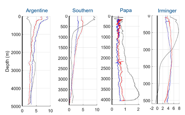
It is often assumed that, at frequencies below inertial, the vertical structure of horizontal velocity and vertical displacement can be reasonably described by a single dynamical mode, e.g. the lowest order flat-bottom baroclinic mode. This is appealing because it would mean that first-order predictions of deep-ocean velocity structure could be determined from knowledge of density and surface currents. However, there is a relative paucity of full ocean depth data to test this idea. A study by Toole et al. (2023) used full ocean depth data from five sites – four of which are Ocean Observatories Initiative (OOI) arrays (Station Papa, Irminger Sea, Argentine Basin and Southern Ocean) – to address the question “does subinertial ocean variability have a dominant vertical structure?”
Data analysis was challenging, because it involved working with gappy records as well as combining information from multiple instruments on different moorings. As noted by the authors, “no single OOI mooring sampled velocity, temperature and salinity over full depth.” Wire-following profiler data from Hybrid Profiler Moorings were combined with ADCP and fixed-depth CTD data from adjacent moorings. While the authors note that “depth-time contour plots of the velocity data from each OOI site clearly reveal the shortcomings of the datasets” they also recognized that despite the shortcomings, “these observations constitute some of the only full-depth observations of horizontal velocity and vertical displacement from the open ocean.”
It was possible to obtain 2-3 years (non-contiguous in some cases) of near-full ocean depth data from each site. Inertial and tidal variability was removed, and the data were filtered over 100 hr (~4 days). Empirical Orthogonal Function (EOF) decomposition was used to identify an orthogonal basis set that described horizontal velocity and vertical displacement. In addition, dynamical modes were determined for three cases: flat bottom, sloping bottom and rough bottom. Note that computing the dynamical modes requires the vertical density profile, which was taken as the mean over each deployment. Analysis was focused on the lowest modes, which accounted for the majority of the variance.
The results (Figure 32) showed that there is an EOF consistent with a dynamical mode at most sites. However, the appropriate dynamical mode is different for each site – no single dynamical accounted for a dominant fraction of variability across all sites. The authors note that differences in bathymetry, stratification and local forcing complicate the picture, with different dynamical processes dominating at different sites. Prior studies (not full ocean depth) that appear to show a “universal” vertical structure may be misleading
This project shows the potential for OOI data, with appropriate processing and analysis, to provide unique insights into ocean structure and dynamics. The researchers have made the combined vertical profile data available to the community on the Woods Hole Open Access Server. The dataset DOI (https://doi.org/10.26025/1912/66426) is also linked here: https://oceanobservatories.org/community-data-tools/community-datasets/.
[caption id="attachment_34586" align="alignnone" width="624"] Mode 1 EOFs for velocity (u, red; v blue; cm/s) and vertical displacement (black, decameters) for OOI arrays at (from left) Argentine Basin, Southern Ocean, Station Papa and Irminger Sea. Adapted from Toole et al., 2023.[/caption]
___________________
References:
Toole, J.M, R.C. Musgrave, E.C. Fine, J.M. Steinberg and R.A. Krishfield, 2023. On the Vertical Structure of Deep-Ocean Subinertial Variability, J. Phys. Oceanogr., 53(12), 2913-2932. DOI: 10.1175/JPO-D-23-0011.1.
Read MoreSubsurface Acoustic Ducts in the Northern California Current System
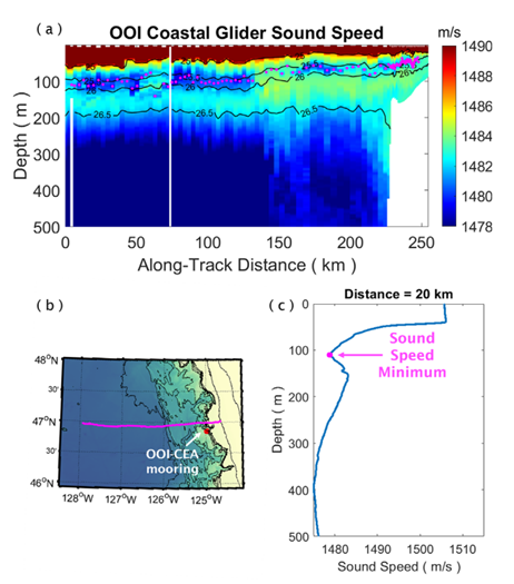
Xu et al.’s analysis of the hydrographic data recorded along the U.S. Pacific Northwest coastline leads to the identification of a secondary subsurface acoustic duct. A numerical simulation based on the sound-speed field determined from OOI Coastal Endurance and APL-UW glider CTD data suggests that the presence of the duct has major impact on sound propagation at a mid-range frequency of 3.5 kHz in the upper ocean (Figure 31). Specifically, the ducting effect is evident in the trapping of sound energy and the consequent reduction in transmission loss within the duct. Glider observations show that the duct is a large-scale phenomenon that extends hundreds of kilometers from the outer continental shelf to regions offshore of the continental slope. The axis of the duct shoals onshore from between 80 and 100 m depth offshore of the continental slope to less than 60 m over the shelf. Analysis of the sound-speed profiles determined from glider CTD data suggests that the prevalence of the duct decreases onshore, from over 40% in regions offshore of the continental slope to less than 5% over the shelf. In addition, analysis of the long-term time series of sound-speed profiles determined from the CTD data recorded over the shelf slope off the Washington Coast suggests that the duct is more prevalent in summer to fall than in winter to spring. Furthermore, examination of concurrent OOI Coastal Endurance Array (Washington Offshore Profiling Mooring) observations of sound speed and flow velocity indicates that the duct observed over the shelf slope is associated with a vertically sheared along-slope velocity profile, characterized by equatorward near-surface flow overlaying poleward subsurface flow.
[caption id="attachment_34581" align="alignnone" width="462"] (adapted from Fig. 3 of Xu et al., 2024) (a) The sound-speed field obtained from the CTD data recorded by an OOI-CEA coastal glider during 06-16 October 2018. The contour lines are potential density (in kg/m3). The magenta dots mark the locations of the local sound-speed minima along the axis of the subsurface duct. (b) The trajectory of the Seaglider. The red dot marks the location of the OOI-CEA Washington Offshore profiler mooring. The bathymetry contour lines mark seafloor depths in 100 m increments between 10 and 500 m and then in 500 m increments between 500 and 3000 m. (c) The vertical sound-speed profile at 20 km along-track distance. The local sound-speed minimum at the axis of the duct is labeled.[/caption]
___________________
References:
Guangyu Xu, Ramsey R. Harcourt, Dajun Tang, Brian T. Hefner, Eric I. Thorsos, John B. Mickett; Subsurface acoustic ducts in the Northern California current system. J. Acoust. Soc. Am. 1 March 2024; 155 (3): 1881–1894. https://doi.org/10.1121/10.0024146
Read More