News
Test Deployments Underway for Pioneer Relocation
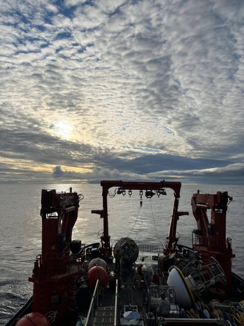
Tuesday February 21, 2023, a team of scientists and engineers from Woods Hole Oceanographic Institution (WHOI) left Charleston, SC aboard the R/V Neil Armstrong to begin test deployments in preparation for the installation of an Ocean Observatories Initiative (OOI) ocean observing system in its new location in the southern Mid-Atlantic Bight (MAB). The science team will deploy two test moorings off the coast of North Carolina, occupying shallow and deep sites of the proposed array. The deployments will supplement computer modeling to ensure the mooring designs perform as expected in the MAB environment. Once the array is fully operational in 2024, the ocean data collected will be available online in near real-time to anyone with an Internet connection.
Ocean observing data helps to track, predict, manage, and adapt to changes in the marine environment. Coastal communities use ocean observing data to prepare for floods and other natural disasters. The instrumented arrays gather physical, chemical, geological, and biological data from the air-sea interface to the seafloor, providing a wealth of information for research and education.
[media-caption path="https://oceanobservatories.org/wp-content/uploads/2023/02/CNSM_buoy_atsea-2-1.png" link="#"]Offshore conditions can be brutal for moorings that remain in the water for six-month deployments. The new location for the OOI’s Coastal Pioneer Array is designed to withstand treacherous conditions, including extreme storms. Credit: ©Woods Hole Oceanographic Institution.[/media-caption]“This new Pioneer Array location in the MAB offers many opportunities for scientists to obtain data to further their research, and will provide better insight into conditions in the area for a variety of stakeholders,“ said Al Plueddemann, Project Scientist for OOI’s Coastal and Global Scale Nodes group at WHOI, which is responsible for operation of the Pioneer Array. “We welcome researchers, educators, and industry members to reach out to us to explore ways we might work together to maximize the usefulness of the data.”
The OOI is funded by the National Science Foundation (NSF) to collect and deliver ocean data in select locations for 25 years or more. This longevity of data collection makes it possible for researchers to identify both short term processes and long-term trends in our changing ocean. The OOI’s Coastal Pioneer Array was designed to be relocatable, and its first deployment was off the coast of New England at the Continental Shelf/Slope interface, where it collected data from 2016 until it was recovered in September 2022. The new location off the coast of North Carolina was chosen by NSF based on input from the science community during a series of NSF-sponsored workshops in 2022.
Dr. Reide Corbett, Executive Director of the Eastern Carolina University’s Coastal Studies Institute (CSI), is enthusiastic about the opportunities the Pioneer Array will bring to the region. “The cross-shelf suite of instrumentation off northeastern North Carolina’s coast is in a region of complex physics and critical ecosystem dynamics that draws interest from many disciplines and creates opportunities for transformational science. This is also in a region with a growing renewable energy sector, including two active offshore wind leases, with opportunities to partner with the agencies involved. The Coastal Studies Institute is excited about the observations that will be made from these instruments, allowing us to better address climate change influences in the coastal ocean, and improve ocean/weather/storm forecasts through data sharing. Beyond just the instruments in the water, the new partnerships and collaborations created as part of this deployment will provide the ability to better engage this socio-economically diverse region, with disadvantaged groups more impacted by sea level rise and climate change compared to many coastal regions. This broad network of partnerships across the region will provide a mechanism to drive knowledge to action,” states Corbett.
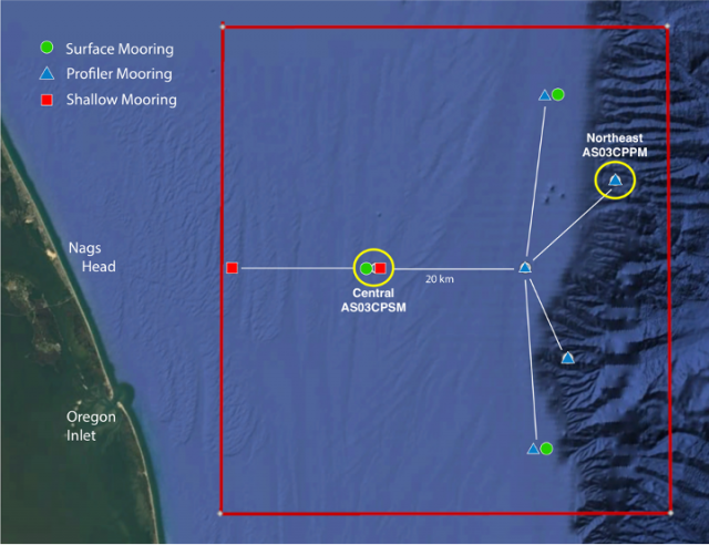
[media-caption path="https://oceanobservatories.org/wp-content/uploads/2023/02/Pioneer-MAB-schematic.png" link="#"]Schematic drawing of the Pioneer MAB moored array to be deployed off the coast of Nags Head, North Carolina. The full array, to be deployed in the spring of 2024, will consist of ten moorings at seven different sites (three sites contain mooring pairs). For the test deployment, one Coastal Surface Mooring will be deployed at the Central site and one Coastal Profiler Mooring will be deployed at the Northeast site.[/media-caption]The new MAB site represents a different environment than the New England Shelf location and offers opportunities to collect data on a variety of cross-disciplinary science topics, including cross-shelf exchange and Gulf Stream influences, land-sea interactions associated with large estuarine systems, a highly productive ecosystem with major fisheries, processes driving biogeochemical cycling and transport, and fresh-water outflows during extreme rain events.
The MAB location is expected to have different wind, wave, and current conditions than the Pioneer Array experienced on the New England Shelf. In addition, deployments in the new location will be in both shallower and deeper water depths than those off the New England coast.
A Coastal Surface Mooring (CSM) will be deployed at 30 meters depth at 35o 57.00’ N, 75o 07.5’ W. The CSM is specifically designed to examine coastal-scale phenomena and withstand the challenging conditions of shallow coastal environments. The Surface Mooring contains instruments attached to a Surface Buoy floating on the sea surface, a Near Surface Instrument Frame 7 meters below the surface, and a Seafloor Multi-Function Node (MFN) located on the seafloor. Additionally, the Surface Buoy contains wind turbines and solar panels for power generation and antennas to transmit data to shore via satellite.
A Coastal Profiler Mooring (CPM) will be deployed at 600 meters depth, 36o 03.80’ N, 74o 44.56’ W. The CPM contains a Wire-Following Profiler that houses instruments. The Wire-Following Profiler moves through the water column along the mooring riser, continuously sampling ocean characteristics from about 23 m below the surface to 23 m above the sea floor. The CPMs also carry an upward-looking Acoustic Doppler Current Profiler to measure ocean currents over the same region of the water column traversed by the profiler.
The test mooring data will be evaluated during the deployment and after recovery to determine whether any modifications are needed to the mooring designs. The plan is to deploy the full array in the spring 2024.
An update on the Pioneer Array relocation is planned for April 20 at 6 pm at the Coastal Studies Institute on East Carolina University’s Outer Banks Campus. Contributing to the CSI “Science on the Sound” lecture series, WHOI’s Dr. Plueddemann will discuss the Pioneer Array infrastructure, instrumentation, and what is planned for its upcoming move off the North Carolina coast. The event is free and open to the public. For those unable to attend, the program will be live-streamed, as well as archived for later viewing, on the CSI YouTube Channel.
[media-caption path="https://oceanobservatories.org/wp-content/uploads/2023/02/A-Frame.png" link="#"]An A-frame at the stern of the ship is used to lift an OOI Coastal Surface Mooring into the water at the start of the deployment. A team secures guidelines to ensure its movements are controlled. Credit: Darlene Trew Crist © WHOI.[/media-caption] [media-caption path="https://oceanobservatories.org/wp-content/uploads/2023/02/DSC0418-scaled.jpg" link="#"]Surface Mooring Recovery operations. Credit: Deidre Emrich © WHOI.[/media-caption]
Read More
Data Explorer Receives Environmental Business Journal Award

The Environmental Business Journal (EBJ) recognized the Ocean Observatories Initiative’s (OOI) Data Explorer’s ability to manage and visualize data with one of its annual awards for Information Technology.
Tetra Tech will accept the award at the EBJ awards ceremony in March 2023 for its role in designing open-source software to support the management, accessibility, and visualization of ocean data. Axiom Data Science, a Tetra Tech company, worked with the OOI Cyberinfrastructure team to develop both front-end and back-end systems for data management and visualization of OOI data feeds.
The OOI, funded by the National Science Foundation, delivers real-time data from sensors in the Atlantic and Pacific Oceans to address critical questions regarding the world’s oceans. Axiom Data Science played a foundational role in designing and operationalizing the Data Explorer, the primary gateway for discovering, visualizing, and accessing OOI data. The Data Explorer makes it possible to search across data points, download full datasets, and compare datasets across regions and disciplines for more than 900 instruments in near real-time. In 2022, Axiom Data Science upgraded the OOI cyberinfrastructure to improve the OOI’s ability to serve ultra-high resolution data streams from next generation ocean instrumentation that span the ocean floor to the sea surface.
“We are honored to have worked with Axiom Data Science to make OOI’s vast amount of data accessible and useable and congratulate them on this recognition of their exceptional work,” said Jeffrey Glatstein, OOI’s Data Delivery Lead and Senior Manager of Cyberinfrastructure. “The capabilities of Data Explorer are only beginning to be realized and will serve the ocean community for years to come.”
Read More
Visit to West Coast OOI Facilities
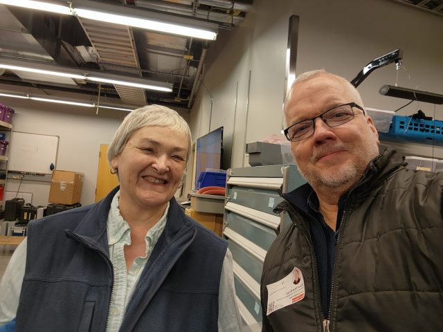
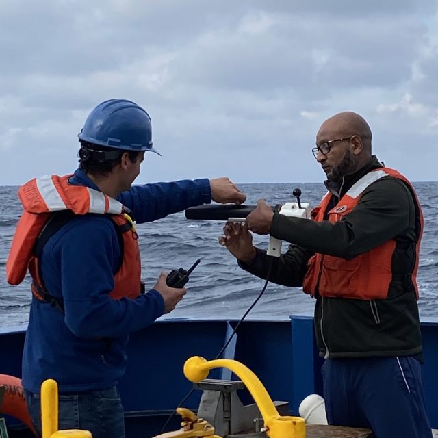
A group of Ocean Observatories Initiative (OOI) leaders visited OOI facilities at Oregon State University and the University of Washington last week to get a first-hand look at operations of the Coastal Endurance Array and Regional Cabled Array, respectively. National Science Foundation Program Director George Voulgaris, OOI Principal Investigator Jim Edson and Senior Program Manager Paul Matthias spent five days on the road meeting with their OOI west coast colleagues. The trip was designed to give recently appointed Voulgaris an opportunity to inspect the infrastructure and meet team members who keep the Coastal Endurance and Regional Cabled Arrays operational and reporting back data around the clock. Edson and Matthias seized the opportunity to meet in person with colleagues who they routinely see on the screen.
The following provides a glimpse of some of the activities that occurred during the trip:
[media-caption path="https://oceanobservatories.org/wp-content/uploads/2023/02/20230207_140014.jpg" link="#"]Grant Dunn, Mechanical Engineer with the Electronic & Photonic Systems Department at UW-APL (left) describes the level-wind system on the RCA profiler mooring to Dr. George Voulgaris during a tour of the RCA laboratory facilities at the University of Washington as RCA Project Manager Brian Ittig looks on. Credit: Paul K. Matthias © WHOI.[/media-caption] [media-caption path="https://oceanobservatories.org/wp-content/uploads/2023/02/20230207_144911.jpg" link="#"]Regional Cabled Array Principal Investigator Deborah Kelley (left) and OOI Senior Program Manager Paul Matthias take a selfie to commemorate their in-person visit during a tour of the RCA facilities at the University of Washington. Credit: Paul K. Matthias © WHOI.[/media-caption] [media-caption path="https://oceanobservatories.org/wp-content/uploads/2023/02/20230207_141656.jpg" link="#"]NSF Program Director George Voulgaris (from left), OOI Principal Investigator Jim Edson look on as Regional Cabled Array technicians Grant Dunn, Mechanical Engineer with the Electronic & Photonic Systems Department at UW-APL, and RCA Chief Engineer Chuck McGuire explain the engineering associated with the RCA profiler mooring during a tour of RCA’s facilities at the University of Washington. Credit: Paul K. Matthias © WHOI.[/media-caption] [media-caption path="https://oceanobservatories.org/wp-content/uploads/2023/02/20230209_123758.jpg" link="#"]NSF Program Director George Voulgaris (left) asks OSU technician Jonathan Whitefield questions about glider operations that provide critical water column data around the moorings of the Coastal Endurance Array. Credit: Paul K. Matthias © WHOI.[/media-caption] [media-caption path="https://oceanobservatories.org/wp-content/uploads/2023/02/20230207_112718.jpg" link="#"]NSF Program Director George Voulgaris (foreground) and RCA Chief Engineer Chuck McGuire discuss the RCA data monitoring systems as OOI PI Jim Edson points to real-time data on the screen being relayed by instrumentation on the Regional Cabled Array. Credit: Paul K. Matthias © WHOI.[/media-caption] [media-caption path="https://oceanobservatories.org/wp-content/uploads/2023/02/20230209_130353.jpg" link="#"]NSF Program Director George Voulgaris (left) gets a hands-on look at the multiple instruments contained on multi-function node that will sit on the bottom of the ocean floor for six months collecting data for the Coastal Endurance Array. Coastal Endurance Array Principal Investigator Ed Dever (middle) and Project Manager Jonathan Fram the functionality of each instrument during the visit to Oregon State University. Credit: Paul K. Matthias © WHOI.[/media-caption]
Read More
Captain Eric Haroldson: 20 Years Aboard the Thompson
20+ Years on the Thompson; A Decade as Captain
Captain Eric Haroldson has lived half of his professional life as a captain aboard the R/V Thomas G. Thompson, which is operated by the School of Oceanography at the University of Washington. With a schedule of three months on, three months off, Haroldson spends roughly half his life at sea each year. And, when he returns to the vessel after three months on terra firma, he said, “The weirdest thing is that I can walk onto the ship after being away for three months and stand in the stair tower just after the galley. Same sounds same smells, everything’s the same. I click right back into it. It’s like I’ve never been gone.” Haroldson’s adjustment to land isn’t as smooth. He finds he needs to adjust to driving a car again and needs to have ceiling fans in his home to mimic the white and perpetual noise of the ship.
While onboard, Haroldson oversees offers 20 officers and crew, two marine technicians, and up to 36 scientists, depending upon the nature of the expedition. At home, he spends time making improvements to the home he built for himself in the woods.
In January, 2023, Haroldson marked a decade at the helm of the R/V Thompson. His journey started in the early 1980s, when he occasionally went to sea as part of the requirements for school and marine-related jobs. The seagoing bug finally hit him in full force in 1989, when he entered the California Maritime Academy. Four years later, he graduated with a third mates’ license and began a career focused on oil industry work.
His first job as a licensed officer was on an oil spill response vessel. After that, he sailed on oil tankers as a third mate. After the company he was working for was sold, he met some folks from Scripps Institution of Oceanography, which moved his career in the direction of oceanographic research. Haroldson sailed as third mate on a couple of Scripps’ ships, until the R/V Thompson needed someone to fill in for a couple of months in 1999. “That couple of months turned into 20 or something here, “ he joked.
Haroldson worked his way up to captain in a traditional way, starting as a third mate. After spending 365 days at sea, he was eligible to test to move up as a second mate. After another 365 days at sea, he tested for chief mate. With another 365 days at sea as chief mate and lots of additional classes and learning experiences, the next step was a master’s license, and ultimately followed by a captain’s license. Each step on the journey requires hands-on sea experience, as well as successfully learning (and passing) the requirements of the next job up the ladder with a host of new, different responsibilities.
Once Haroldson left the oil industry, he never looked back. “Not only is the work better aboard a research vessel, it’s more varied and interesting, not to mention important, but the variety is particularly important for those of us who have spent so much of their lives on the water.
He compared the work aboard an oil tanker – which ran between Valdez, Alaska and Exxon Benica in San Francisco Bay. “It was eight days to Valdez, a day and a half to load, followed by an eight-day journey to Benica, where we’d spend a day and a half offloading. The cycle constantly repeated itself and we could literally set our clock by it,” Haroldson explained. “When I started sailing oceanographic vessels, it was okay, well, this is more interesting, I was seeing something different every day. The variety of it gives the job definition and we manage the ship much differently.”
“As captain of a research vessel, we have the opportunity to work along-side scientists, which is great,” he added. “We sit around a table and together we figure out “how do we do this? Or how do we approach this? So there is not only the importance of the work that is happening onboard, but we have the opportunity to see the bigger picture of why this work is so important.”
[media-caption path="https://oceanobservatories.org/wp-content/uploads/2023/02/Screen-Shot-2023-02-10-at-3.05.25-PM.jpeg" link="#"]Captain Eric Haroldson looks out from the R/V Thompson’s bridge windows as Third Mate Todd Schwartz and AB Pam Blusk steer the ship thru the icy waters off Antarctica. Credit: Instagram.[/media-caption]While the ocean itself still presents the same challenges as it did 20 years ago when Haroldson began his journey, he has witnessed a lot of ancillary changes in how and where the ocean is used. “Ports are more interesting, with a greater variety of types of boats and people are fishing in areas where people didn’t fish ten years ago or so.” Haroldson added. He’s also witnessed the evolution of a more diverse crew, with women having a greater presence than in his early days aboard the oil tankers. At times, he’s sailed the R/V Thompson when all of the mates were female, and at other times, the crew has been more than half women.
Haroldson clearly relishes his job and provides a sense of safety, security, and humor while onboard. His greatest challenge seems to be always having to be two-steps ahead of everything in a realm where the rules and the physical condition under which he must safely operate his vessel are perpetually changing. This is no small task.
Sailing in and out of port at Newport Oregon is an example of staying two steps ahead of the game. Haroldson has to ensure that all ship operations are executed in a timely way so they can arrive at Newport at high tide slack water in daylight to avoid running aground. This requirement also provides the captain some flexibility in dictating scheduling. “If the weather is picking up and it will take a couple of hours to get to the site, there’s a decision to be made. Do you want to leave the dock and go out there and bounced around? Or does it make more sense to delay a little bit to the make the passage easier and more pleasant for everyone on board?”
Staffing creates another challenge onboard. Much like airline personnel, ship crew are limited in the number of hours they are allowed on the job. The maximum a crew member can work in a day is 15 hours. But if they work that full 15 hours, then for the next two days, they are only allowed to work up to a total of 20 hours. “We always have to be aware of the crew’s schedules and operate within these guidelines that help ensure safe operations.”
In looking back at his life on the water, Haroldson was enthusiastic about his path and optimistic of others who may follow him on a life well-lived a sea. “It makes for a challenging and rewarding life, and in some cases, there really are opportunities to travel and see the world. And, as long as one likes people and doesn’t mind being part of a community, it can be extremely gratifying—makes one appreciate life on and off the water.”
Read More
Bio-Optics Sensor Summer School Applications Open
Are you interested in using OOI’s optical attenuation and absorption data in your research? Have you ever faced challenges finding and interpreting this type of data? If so, we hope you will consider applying for the 2023 OOI Bio-Optics Sensor Summer School.
The Ocean Observatories Initiative Facility Board (OOIFB) will host the summer school on July 17-21, 2023 on the campus of Oregon State University in Corvallis, OR. The course will focus on learning how to analyze and interpret the Sea-Bird AC-S measurements of optical attenuation and absorption. The AC-S is a hyperspectral instrument used to characterize the way seawater absorbs and scatters light and total scattering can be derived for living and detrital particles in the ocean. The OOI Program deploys the Sea-Bird AC-S on most of the OOI platforms, including coastal, cabled, and high latitude moorings.
Marine phytoplankton play an important role in ocean ecology and global biogeochemical cycles. The optical attenuation and absorption data from the AC-S provides information on the relative biomass of different phytoplankton size classes and phytoplankton functional types. In addition, other biogeochemical proxies, such as particulate organic carbon, may be estimated. The AC-S data also may be used to validate remote sensing measurements. These observations will be useful in addressing science questions covered by several OOI research themes including:
- Climate Variability, Ocean Circulation, and Ecosystems.
- Coastal Ocean Dynamics and Ecosystems.
- Turbulent Mixing and Biophysical Interactions.
About 25 advanced graduate students, post-doctoral fellows, and early career scientists will be selected as participants for the summer school. Other career level researchers will be considered, based on space availability. Participants should have a general understanding of oceanography/biology. Only applicants from U.S institutions can be considered. Participation will be in-person only and all selected students must be available to attend all days of the course. Funding for reimbursement of travel expenses, accommodations, and meals is offered.
Additional details about the summer school program, as well as a link to the application form are available here.
Please submit your application by the end of the day on February 28, 2023. Selections and notifications will be made in March.
OOI Data Classroom at Sea
Ocean Data Labs researcher Sage Lichtenwalner took his data capabilities to the waves, so to speak, as he shared how Ocean Observatories Initiative (OOI) data can be used in the classroom with researchers and teachers aboard the R/V Neil Armstrong in early January. The OOI is funded by the National Science Foundation to collect ocean observations from five scientifically important sites in both the Atlantic and Pacific and make the data available over the internet for research and education.
Lichtenwalner, a research programmer at Rutgers University, was asked to join the cruise as part of an effort to build partnerships and future opportunities between STEMSEAS (Science, Technology, Engineering and Math Student Experiences Aboard Ships) and several Historically Black Colleges and Universities (HBCUs). The cruise was designed to align with STEMSEAS’ objectives and be both immersive and experiential for 12 participants from ten institutions, including six HCBUs. The idea was for faculty to experience the cruise as students on other STEMSEAS expeditions do, and to take back what they learned from their onboard experiences to share with their students and classes. They traveled from Woods Hole, MA to Pensacola, Fla., from January 3-11, 2023.
Lichtenwalner provided participants with practical, hands-on ways to integrate OOI data into their courses. During the eight-day cruise, Lichtenwalner gave four presentations to the group, including a demonstration about how they can use the OOI Data Labs Manual in their classes. “The OOI Data Labs Manual is an easy, accessible way to use real ocean data to teach oceanographic concepts,” he said. “Educators have found that the real-time nature of OOI data inspires students, making them more engaged with the data because of their timeliness and relevance.”
Lichtenwalner’s presentations were part of a series of talks given by the STEMSEAS team and HBCU participants, which included hands-on activities and resources to build students’ problem-solving and scientific thinking skills. Participants also shared their research and teaching strategies to foster collaborative discussions.
[media-caption path="/wp-content/uploads/2023/01/group-shot.png" link="#"]Spending eight days at sea together provided participants with plenty of hands-on learning about sampling at sea, as well as opportunities to share research and teaching strategies they use when on land.[/media-caption]
Onboard the R/V Neil Armstrong, Dr. Magdalena Andres, a physical oceanographer at Woods Hole Oceanographic Institution and co-Principal Investigator of the PEACH program, which is investigating physical processes that drive exchanges between the shelf and deep ocean at Cape Hatteras, served as chief scientist on the cruise. She put the visiting team to work, helping deploy instruments and make underway measurements as part of the “SWOT Adopt a Crossover Field Campaign—Cape Hatteras.” The project, funded by NASA’s Jet Propulsion Laboratory, falls under the umbrella of the Surface Water Ocean Topography (SWOT) Adopt a Crossover Consortium. Andres is part of a multi-institution research team that has “adopted” the site east of Cape Hatteras near the OOI Mid-Atlantic Bite array site, both to advance the community’s dynamical understanding of this key oceanographic region and to help validate measurements provided by the SWOT satellite which launched in December 2022. “SWOT promises to revolutionize our understanding of earth’s surface water. It’s exciting to have the STEMSEAS, HBCU, and Ocean Data Labs participants working side-by-side with the project’s scientists, engineers, students, and technicians on this forefront of ocean observing,” explained Andres.
[media-caption path="/wp-content/uploads/2023/01/IMG_5670-2-scaled.jpeg" link="#"]Loretta Williams Gurnell (right), founder of the SUPERGirls SHINE Foundation, is learning about atmospheric turbulence with a hands-on demonstration led by Dr. Alex Gonzalez from the Physical Oceanography department at the Woods Hole Oceanographic Institution. Alex is part of the NSF-supported DIYnamics Team, https://diynamics.github.io/pages/about.html, which is working to provide access to affordable materials for geoscience teaching demonstrations.[/media-caption]
While onboard, Andres had the team assist her in deploying current and pressure sensing inverted echo sounders (CPIESs) and XBTs (expendable bathythermographs), as well as collecting measurements with the ship’s CTD (conductivity, temperature, depth) profiler. CTDs measure vertical profiles of conductivity (a proxy for salinity) and temperature. XBTs collect profiles of temperature. CPIESs measure bottom pressure and vertical acoustic travel time data (a proxy for temperature and salinity profiles) and near bottom current measurements (velocity of ocean water). The CPIESs were left in place to collect data over the next 18 months.
In 2024, the OOI Pioneer Array will move to the Mid-Atlantic, not far from where the cruise deployed the CPIES and collected CTD casts. To prepare participants for future potential educational applications of OOI CTDs and other instruments in the area, Lichtenwalner made quick plots of the data collected along the way. “Doing real-time plotting to support operations is actually how I got started in oceanography, so it’s been fun to re-live that experience, while also introducing a new group of professors and educators to the power of using ocean data in real-life and in the classroom.”
Read More
AGU Lightning Talks
Here is an opportunity to hear some of the latest findings and research in the works based on OOI data. Researcher presented their findings in one-minute lightning talks at the AGU Fall Meeting December 12, 2022 during OOIFB’s Town Hall. The presenters are listed by topic and time that they appear on the video. For questions, please don’t hesitate to contact the researchers directly.
- 0:10: Cesar Savage – Woods Hole Oceanographic Institution (virtual)
- 2:16: Artash Nath – MonitorMyOcean.com (virtual)
- 4:00: Karen Bemis – Rutgers, The State University of New Jersey
- 5:45: Ettore Biondi – California Institute of Technology
- 7:46: Amy Bower – Woods Hole Oceanographic Institution
- 11:53: Marine Denolle – University of Washington
- 14:05: Jiaqi Fang – California Institution of Technology
- 15:45: Aleck Wang – Woods Hole Oceanographic Institution
Read More
Alex Wick: Conducting Sea-going Operations
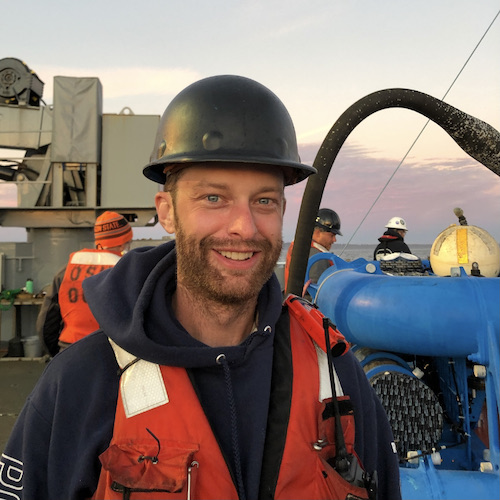
OOI Coastal Endurance Array Deck Lead Alex Wick has been working on ships for more than a decade. He is a classic example of learning the ropes from the bottom up. After receiving a degree in marine biology from the University of Santa Cruz, he took some scuba diving lessons, but really didn’t know what he wanted to do.
Wick started his journey aboard ships in 2012 sorting tools for a marine technician onboard the R/V Point Sur, out of Moss Landing, California. When offered the job, he had no idea what he was getting into. He showed up in shorts, street shoes, with no personal protective gear (PPE) at all, and no at-sea experience.
But he learned quickly and advanced from sorting sockets to needle-gunning the deck, which involves removing all of the old paint with a needle gun before applying a new coat of paint. This activity was when Wick was given his first set of PPE – safety glasses, knee pads, hard hat, and gloves – which gave him a real understanding of their importance during five days of back-breaking work.
[media-caption path="/wp-content/uploads/2023/01/Alex.jpeg" link="#"]Alex Wick has been deck lead for Endurance Operations since 2018. Credit: Darlene Trew Crist ©WHOI.[/media-caption]
Wick started repainting the deck of the boat. The captain, at the time, recognized Wick’s work ethic and dedication and continued to expose him to shipboard duties. From one cruise as a deck hand, he advanced to an 84-day expedition to Antarctica. He jokes that at the time he didn’t even know how to use a ratchet strap, which is widely used to secure heavy equipment on ships and elsewhere.
“The captain told me to secure a small boat under the A-frame,” said Wick. “I had no idea how to do, but figured it out. With one day of oceanographic experience under my belt, I was off to Antarctica.” As it turned out, it was the best possible hands-on learning experience for Wick, which ultimately led to him spending about 500 days at sea and his role with the Endurance Array team today.
“There was nothing like driving a boat in Antarctica with a guy with a crossbow on the bow of the boat directing me around chasing Minke whales,” added Wick. “We would come up alongside one of them, shoot a crossbow bolt into its dorsal fin to retrieve a bio-sample. I thought it was the coolest thing ever.”
This Antarctica expedition provided Wick with the foundational knowledge he now uses aboard the R/V Thomas G. Thompson during bi-annual recovery and deployment expeditions for the Coastal Endurance Array. His time on the Point Sur taught him how to run winches, use the A and J frames, which support the lifting of heavy equipment in and out of the ocean, and most importantly, how to work on a ship in a safe manner.
After Antarctica, Wick spent six years as a deck hand and marine technician, where he developed an innate understanding of how all the pieces move on deck. Jonathan Fram, who often serves as chief scientist for the Endurance expeditions likens Wick to a symphony conductor. “He directs the operations while always having an eye on each member of the ‘orchestra’ and what they should be doing at certain times. This orchestration is critical to getting the heavy equipment we deal with on and off board without incident.”
Wick moved to Oregon State University when his wife was accepted into a PhD program there. He was hired on as a marine technician on the R/V Oceanus, where he sailed for up to 100 days a year. But, a man of many interests, Wick grew tired of being away from home for such long stretches. He missed his family, mountain bike, fishing, and other activities afforded by living in Oregon. He applied for the job as deck lead with the Endurance Array team and has been on the job since December 2018.
His first trip to the dock in Newport after a fall Endurance expedition, where he saw the massive amount of equipment moved on and off the ship and in and out of the water, provided Wick with his leadership philosophy.
“I think that the person running the deck should be basically completely hands off. That way, we are able to actually observe everything and see the bigger picture of what’s happening,” said Wick. “As we’re doing recoveries or deployments, I’m always thinking of the next pieces of the puzzle. I want the folks on the back deck and on the bridge to know what to expect, so everyone knows what’s ahead and can plan for what they’re going to be doing.”
From the seeds of his earliest experience aboard the R/V Point Sur, Wick is totally committed to overseeing a safe operation. “The deck lead is responsible for everyone’s safety and making sure we’re doing things appropriately,” he explained. “Sure unexpected things can happen, but back deck operations can and should be done safely. I feel a great responsibility for making sure that everybody comes back with all their digits and we all return to shore having successfully completed the job and return to our family and friends.”
Wick’s favorite part of the job is working with the team. He joked, “We are all part of the communal suffering. Doing the same thing together. We have a lot of big toys that we get to play with safely. And, it really is special at sea. It’s cool to see the whales breaching, the dolphins racing the ship, the bioluminescence, and skies filled with stars. No matter how crusty and jaded we might be, it takes a team to put these moorings in the water, and deep down, I think we all really enjoy doing this.”
Wick has served as deck lead for six Endurance expeditions and has overseen the movement, deployment and recovery of 270 tons of scientific equipment. Not a bad record for a kid who started out sorting tools.
[media-caption path="/wp-content/uploads/2023/01/Alex-2.jpeg" link="#"]Wick choreographs the recovery and deployment of the Endurance Array moorings. Credit: Darlene Trew Crist ©WHOI. [/media-caption]
Read More
Science Highlights
Researchers from around the globe are using OOI data to identify short-term changes and long-term trends in the changing global ocean.
The Science Highlights included in the report below were compiled from quarterly reports submitted by the Ocean Observatories Initiative to the National Science Foundation from 2020-2022. They represent only a fraction of the scientific findings that are based on OOI data. A complete list of peer-reviewed publications based on OOI data can be found here.
[embed]https://issuu.com/oceanobservatoriesinitiative/docs/ooi_science_highlights_autosaved_.pptx?fr=sNzM0ZjQ2ODUxNTQ[/embed]
Read More
A Visual Report of OOI in 2022