
Posts Tagged ‘Coastal and Global Scale Nodes’
Shelfbreak Jet Influence on Coastal Sea Level
Flooding and shoreline erosion are increasing threats to coastal communities. Coastal sea levels are influenced by multiple factors, including mean sea level rise, tides, storm surges, river outflow, and waves. A recent paper by Camargo et al. (2025) focused on the extent to which offshore circulation, in particular the shelfbreak jet on the New England shelf, contributed to sea level variability over the period 2014 – 2022. They found that roughly 30% of sea level variance during storm surges can be attributed to the shelfbreak jet.
The authors used a variety of data sets, including tide gauge stations along the New England coastline from Boston, MA to Atlantic City, NJ, wind stress from the ECMWF ERA-5 reanalysis, and shelfbreak jet transport from the OOI Pioneer Array. The jet transport was estimated using upward-looking ADCP data from the Central Inshore, Central, and Central Offshore moorings. The methodology and results are described in Carmargo et al., 2024 and the jet transport data set is available in Zenodo (Carmago, 2024). The data were de-tided and then band-pass filtered (1-15 days) to isolate the storm-surge component of sea level variability. Coherence between coastal sea level and jet transport for 1-15 day periods was established by Carmago et al. (2024).
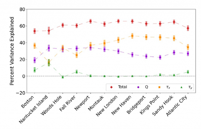
[caption id="attachment_37571" align="alignnone" width="975"]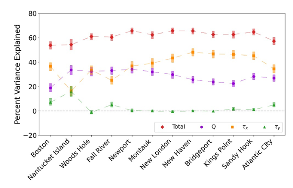 Percent of storm surge variance explained by the regression model (red) and for individual parameters: shelfbreak jet (purple), zonal wind stress (orange), and meridional wind stress (green). Tide gauge stations are ordered from north to south along the coastline. From Camargo et al., 2025.[/caption]
The influence of jet transport and two components of wind stress (zonal and meridional) on storm surge was evaluated by means of a linear regression model that determined the regression coefficients for each parameter. The regression was run for each tide station using the previously computed jet transport and the ERA-5 wind stress closest to each station. Overall, the regression model explained about 60% of the storm surge variance, with jet transport and zonal wind stress explaining 28% and 38%, respectively. There was modest along-coast variability in the variance explained by each parameter (Figure 3): Variance explained by zonal wind stress tended to increase from NE to SW along the coast (Fall River to Bridgeport), while variance explained by the jet tended to decrease. The wind stress impact was identified as due to either onshore or downwelling-favorable winds. The jet impact was due to changes in the cross-shelf pressure gradient associated with the geostrophically-balanced currentCase studies for specific synoptic events highlight the complexity of coastal storm surge events and the broad suite of observational tools necessary to determine the influence of different mechanisms. The authors note that simple storm surge models will not capture the influence of offshore currents like the shelfbreak jet, and that such influence is likely to be found elsewhere on the US east and west coast.
___________________
References:
Camargo, C.M.L., C.G. Piecuch and B. Raubenheimer, 2025. Do ocean dynamics contribute to coastal floods? A case study of the shelfbreak jet and coastal sea level along southern New England, Earth’s Future, 13, https://doi.org/10.1029/2025EF006708.
Camargo, C. M. L. (2024). Shelfbreak jet transport from OOI pioneer [Dataset]. https://doi.org/10.5281/zenodo.10814048.
Camargo, C. M. L., Piecuch, C. G., & Raubenheimer, B. (2024). From shelfbreak to shoreline: Coastal sea level and local ocean dynamics in the Northwest Atlantic. Geophysical Research Letters, 51(14), e2024GL109583. https://doi.org/10.1029/2024GL109583 .
Read MoreA Carbon Budget for the Upper Mesopelagic Zone

(Adapted from Stephens et al., 2025)
Upper ocean carbon budgets are difficult to constrain, and those for the mesopelagic zone come with particular challenges. A recent paper by Stephens et al. (2025) took on the challenge of a comprehensive carbon system budget for the upper mesopelagic zone (100-500 m) based on data from the EXport Processes in the Ocean from RemoTe Sensing (EXPORTS) program (Siegel et al., 2016). The 2018 EXPORTS field campaign was conducted at Ocean Station Papa in the Northeast Pacific to take advantage of the relatively modest surface forcing, shallow summer mixed layer, tightly coupled food web, and low mesoscale kinetic energy. Nevertheless, the study found that a steady-state assumption for the carbon system was likely not appropriate.
Measuring organic carbon supply and demand is challenging due to a variety of factors. Supply includes sinking particles, migrating zooplankton and fish, disaggregation, mixing and subduction. Demand comes primarily from bacteria and zooplankton. Measurement methods for each supply and demand term have errors, conversions to rates have uncertainties, and each process being measured may have a unique timescale over which a rate integration makes sense. EXPORTS was notable for increasing the number and variety of measurements available for monitoring the mesopelagic carbon budget. Stephens et al. take advantage of this by combining multiple measurement methods, quantifying errors and applying statistical methods for error analysis.
The authors used observations from multiple sources. Near-surface data came from the PMEL Station Papa surface mooring. Shipboard profile data come from two ships operating during the EXPORTS field campaign as well as the OOI Station Papa cruise in 2018. Additional water column data came from two OOI Slocum gliders, one EXPORTS-operated Seaglider, and BGC Argo floats. The authors examined each carbon supply and demand estimate, calculating an uncertainty and discussing potential limitations (Stephens et al., Table 1). A Monte Carlo approach was used to assess overall uncertainty in supply and demand terms, resulting in the conclusion that supply was insufficient to meet demand (e.g. Fig. 1 below). The error analysis allowed the authors to conclude that the mismatch was not the result of problems in estimating supply or demand, but rather a problem with the assumption that supply and demand would balance within the analysis period. In other words, the system was not in steady state.
This project highlights the complexity of the carbon system in the upper ocean and the broad suite of observational tools necessary to address the carbon budget. The authors make three specific recommendations for improved quantification of the biological carbon pump: including the relevant midwater processes, capturing the range of relevant timescales, and providing redundancy in methodology.
[caption id="attachment_37368" align="alignnone" width="928"]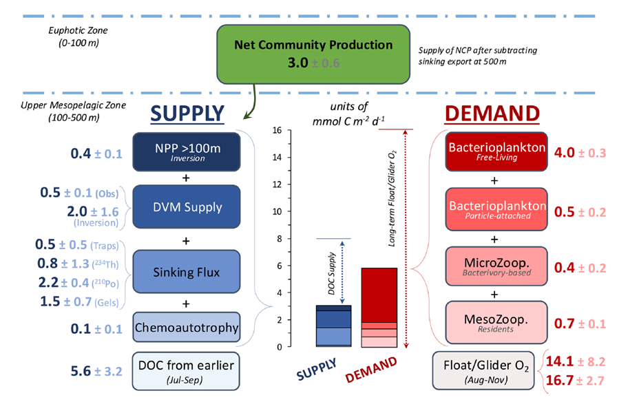 Assessment of the organic carbon budget in the upper mesopelagic zone during EXPORTS. Estimated individual contributions to supply (left) and demand (right) are provided along with error estimates. Terms with multiple measurement methods (far left, far right) were averaged. The center panel shows the cumulative supply and demand relative to a vertical scale in units of mmol C per (m^2 day). From Stephens et al., 2025.[/caption]
___________________
References:
Stephens, B.M., and 20 co-authors, 2025. An upper-mesopelagic-zone carbon budget for the subarctic North Pacific, Biogeosciences, 22, 3301-3328, https://doi.org/10.5194/bg-22-3301-2025.
Siegel, D.A., K.O. Buesseler, M.J. Behrenfeld, C.R. Benitez-Nelson, E. Boss, M.A. Brzezinski, A. Burd, C.A. Carlson, E.A. D’Asaro, S.C. Doney, M.J. Perry, R.H.R. Stanley and D.K. Steinberg, 2016. Prediction of the Export and Fate of Global Ocean Net Primary Production: The EXPORTS Science Plan, Front. Mar. Sci., 3:22, https://doi.org/10.3389/fmars.2016.00022.
Read More
The 2019 marine heatwave at Ocean Station Papa
(Adapted from Kohlman et al., 2024)
Marine Heat Waves (MHW; Hobday et al., 2016) are prolonged periods of extreme ocean sea surface temperature (SST) anomalies. MHWs are typically identified in satellite SST and/or ocean color records; subsurface data and interdisciplinary variables are often lacking. Ocean Station Papa (OSP) provided long-term, interdisciplinary, subsurface data to examine the physical and biochemical characteristics of a MHW in the Northeast Pacific.
MHWs may have multi-faceted causes, as well as impacts on primary production and higher trophic levels. A recent paper by Kohlman et al. (2024) examines the 2019 NE Pacific MHW using gridded satellite SST data and in-situ observations from multiple OSP platforms including the NOAA Pacific Marine Environmental Lab (PMEL) surface mooring, two OOI Flanking Moorings, the Applied Physics Lab (U. Washington) waverider mooring and shipboard samples from OOI and the Department of Fisheries and Oceans, Canada.
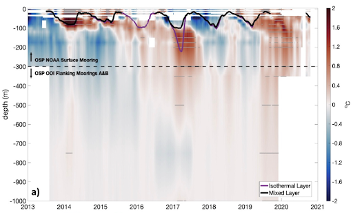
The 2019 MHW was identified in satellite SST data, but the Kohlman et al. study also assessed vertical stratification and the subsurface extent of the temperature signal. The PMEL surface mooring provided temperature and salinity (T/S) down to 300 m. The OOI Flanking Moorings extended the T/S data to 1500 m. The resulting composite time series from 2013-2020 is shown in Fig. 1. Both the extended 2013-2015 MHW and the 2019 MHW are identifiable. Subsurface temperature anomalies during 2013-2014 were strongest above the mixed layer depth (MLD). In the winter and spring of 2017, deeper waters (120–300 m) remained anomalously warm. This anomaly persisted into 2018 due to strong stratification from a fresher surface layer. During the 2019 MHW, anomalously warm waters extended down to 1000 m, whereas the 2013-2015 MHW extended only to about 150 m.
The authors used interdisciplinary data available from Station Papa platforms to assess the drivers and impacts of the 2019 MHW. They found that weaker winds and smaller significant wave height prior to the summer of 2019 created favorable pre-conditioning in the form of an unusually shallow winter MLD. During the MHW, they found that dissolved inorganic carbon and pCO2 decreased, while pH increased. Shipboard samples indicated a decrease in nutrients and an increase in primary productivity. Finally, they speculated that the increased productivity may have had an impact on higher trophic levels – more blue whale calls were recorded in 2019 at Station Papa than normal for Aug-Sep.
This project shows that the characteristics of MHWs are complex. Sustained, multi-disciplinary, subsurface observations are needed to unravel the drivers, pre-conditioning, characteristics, and impacts of these events. Station Papa, among the longest sustained ocean time series sites, is uniquely suited due to the task due to the collaborative observing effort at the site.
[caption id="attachment_37120" align="alignnone" width="512"] Figure 1. Subsurface temperature anomalies at Staton Papa during 2013-2020. Data from the surface to 300 m are from the PMEL surface mooring. Data below 300 m are from the OOI Flanking Moorings. Anomalies are relative to the 1999-2020 Argo climatology. The density-based mixed layer depth (black) and isothermal depth (purple) are overlaid. From Kohlman et al., 2024.[/caption]
___________________
References:
Hobday, A.J., Alexander, L.V., Perkins, S.E., Smale, D.A., Straub, S.C., Oliver, E.C.J., et al. (2016). A hierarchical approach to defining marine heatwaves. Prog. Oceanog., 141(0079–6611), 227–238. https://doi.org/10.1016/j.pocean.2015.12.014.
Kohlman, C., Cronin, M.F., Dziak, R., Mellinger, D.K., Sutton, A., Galbraith, M., et al. (2024). The 2019 marine heatwave at Ocean Station Papa: A multi‐disciplinary assessment of ocean conditions and impacts on marine ecosystems. J. Geophys. Res., 129, e2023JC020167. https://doi.org/10.1029/2023JC020167.
Read MoreSAR Imagery Detects Atmospheric Stratification
(Adapted from Stopa et al., 2024)
There is interest in using satellite-based Synthetic Aperture Radar (SAR) imagery to assess phenomena related to atmospheric boundary layer stratification over the ocean. Obtaining such information with high spatial and temporal resolution would advance boundary layer research and would be beneficial to the development of offshore wind energy. However, monitoring marine boundary layer structure remotely is a challenge. A recent paper by Stopa et al. (2024) shows that it is possible to utilize SAR imagery, in conjunction with in-situ meteorology, to characterize boundary layer stratification.
The Central Surface Mooring (CNSM) of the OOI Pioneer New England Shelf Array is located near a region of offshore wind development where SAR imagery is also available. The authors use wind speed, air temperature, and sea surface temperature from the CNSM buoy to estimate the bulk Richardson number (Ri), a measure of marine atmospheric boundary layer stability. OOI quality control flags were used to identify good data, and suspect data were replaced with data from redundant sensors. CNSM data from 2014 – 2021 were used in the analysis.
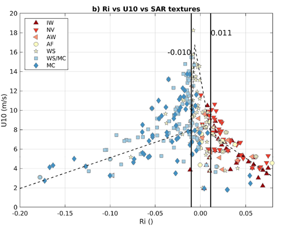
SAR data are commonly used to provide wind speed estimates, but the images also contain rich information about coherent structures in the atmosphere, and those structures correspond to boundary layer stratification regimes (Stopa et al., 2022). The Stopa et al., (2024) study used European Space Agency Sentinel-1 C-band SAR wave mode (S1 WV) imagery spanning the region of the NES Pioneer Array. SAR Images in 20 x 20 km regions were visually examined and classified based on observed “signatures” of atmospheric phenomena. Of particular interest for this study were signatures indicative of waves, rolls/streaks and convection (Table 1).
The relationship of SAR image classes to wind speed and atmospheric stability was examined by plotting the classified data set vs Ri and U10 (Figure 1). U10 shows a change in slope near neutral stratification (Ri = 0) with indications of a Ri-U10 relationship at higher and lower Ri. Of interest is the appearance of Ri boundaries denoting transitions between unstable (Ri < -0.01), neutral, and stable (Ri > 0.01) regimes. Rolls, streaks and convection dominate the unstable regime, while waves dominate the stable regime. In other words, classification of the SAR images provides information about atmospheric stratification.
This project shows the power of combining remote sensing with long-term, in-situ meteorological measurements to gain insights that neither could provide alone. The authors note that when satellite data are available, the SAR-based determination of boundary layer structure can be used over broad areas and long times, and is more efficient than direct measurements such as buoy-based LIDAR.
Table 1: Atmospheric signatures in SAR imagery
| Class | Phenomena |
| NV | Lack of rolls or cells |
| AW | Atmospheric gravity waves |
| IW | Oceanic internal gravity waves |
| WS | Rolls or wind streaks |
| MC | Microscale convection |
| WS/MC | Combined WS/MC |
Figure 1. SAR image classes shown as different symbols) vs. Richardson number (Ri) and ten meter wind speed (U10). Note the regime transitions near Ri = -0.01 and +0.01. From Stopa et al., 2024.[/caption]
___________________
References:
Stopa, J.E., C. Wang, D. Vandemark, R.C. Foster, A. Mouche, and B. Chapron, (2022). Automated Global Classification of Surface Layer Stratification Using High-Resolution Sea Surface Roughness Measurements by Satellite Synthetic Aperture Radar,” Geophysical Research Letters 49(12), e2022GL098686.
Stopa, J.E., D. Vandemark, R. Foster, M. Emond, A. Mouche, and B. Chapron (2024). Characterizing the Atmospheric Boundary Layer for Offshore Wind Energy Using Synthetic Aperture Radar Imagery. Wind Energy, 27:1340–1352, https://doi.org/10.1002/we.2933.
Read MoreSalinification of the Cold Pool on the New England Shelf

(Adapted from Taenzer et al., 2025)
The continental shelf within the Mid-Atlantic Bight is cooled and mixed vertically in the winter. This relatively cold, fresh water is trapped below the seasonally-warming surface layer, retaining its properties as a subsurface “cold pool” throughout most of the spring and summer. The cold pool is important for regional ecosystems, serving as a cold-water habitat and a nutrient reservoir for the continental shelf. It is known that the cold pool warms and shrinks in volume as a result of advective fluxes and heat exchange with surrounding waters. A recent paper by Taenzer et al. (2025) shows for the first time that the cold pool is also subject to salt fluxes and increases significantly in salinity from April to October.
The Pioneer New England Shelf (NES) inshore moorings (ISSM and PMUI) are positioned shoreward of the shelfbreak front and sample conditions on the outer continental shelf where the cold pool can be identified. The authors extracted data from these two moorings from a quality-controlled data set containing timeseries of hydrographic data (temperature, salinity and pressure) from all of the Pioneer NES moorings on a uniform space-time grid, covering the timeframe from January 2015 through May 2022 (Taenzer et al., 2023). The cold pool study used data from 2 m depth, 7 m depth, and 2 m above the bottom on ISSM and from roughly 28 m to 67 m depth on PMUI.
Seven years of data from the Pioneer ISSM and PMUI moorings were used to create a composite annual cycle, which showed that subsurface salinity on the outer shelf consistently increases in the spring and summer. Evaluating the 67 m depth salinity record, and restricting the time period to when the moorings are in the cold pool, resulted in a salinification estimate of 0.18 PSU/month, or ~1 PSU over the six month period (Figure 34a). It was shown that this salinity change could not be explained by a seasonal change in the frontal position.
Isolating the corresponding cold pool region within the New England Shelf and Slope (NESS) model (Chen and He, 2010), and computing a similar multi-year mean, showed a salinification trend nearly identical to that from the observations (Figure 34b). Using the model, it was possible to define a three-dimensional cold pool volume and estimate terms in the cold pool salinity budget. It was found that cross-frontal fluxes transport salt from offshore to the cold pool at a relatively steady rate throughout the year, and that along-shelf advection contributes little to the salinification process. It was argued that the cold pool exhibits two regimes that result in the seasonal salinification: During the winter, vertical mixing is strong, and the cold pool gets replenished with fresh water from the surface layer, which tends to balance the cross-shelf salt flux. During the spring and summer, surface stratification increases, vertical mixing is inhibited, the cold pool is effectively isolated from surface mixing, and the cross-shelf salt flux results in cold pool salinification.
This project shows the importance of long-duration observations in key locations to isolate phenomena that would not be identifiable from a short-term process study. It is notable that the authors undertook a significant quality control effort and created a merged, depth-time gridded data set that was made publicly available. By combining the observations with a high-resolution regional model, the authors were able to examine the cold pool salinity budget and attribute the observed signals to ocean processes.
[caption id="attachment_36391" align="alignnone" width="402"] Figure 34: The seven-year mean annual cycle of continental shelf cold pool salinity from a) Pioneer Array PMUI salinity at 67m depth, b) NESS model salinity for all waters below 10◦C along 70.875 W. The shaded envelope depicts one standard deviation of interannual variability. The salinification trend is from a linear fit during the stratified season (April-October). From Taenzer et al., 2025.[/caption]
___________________
References:
Chen, K., & He, R. (2010). Numerical investigation of the Middle Atlantic Bight Shelfbreak Frontal circulation using a high-resolution ocean hindcast model. J. Physical Oceanog., 40 (5), 949 – 964. doi:10.1175/2009JPO4262.1
Taenzer, L.L., G.G. Gawarkiewicz and A.J. Plueddemann, (2023). Gridded hydrography and bulk air-sea interactions observed by the Ocean Observatory Initiative (OOI) Coastal Pioneer New England Shelf Mooring Array (2015-2022) [data set], Woods Hole Oceanographic Inst., Open Access server, https://doi.org/10.26025/1912/66379.
Taenzer, L.L., K. Chen, A.J. Plueddemann and G.G. Gawarkiewicz, (2025). Seasonal salinification of the US Northeast Continental Shelf cold cool driven by imbalance between cross-shelf fluxes and vertical mixing. J. Geophys. Res., accepted.
Read MoreIrminger Sea Convection and the roles of Atmospheric Forcing and Stratification

The high-latitude North Atlantic, is a region where seasonal convection results in deep water formation, a process critical to the Atlantic Meridional Overturning Circulation (AMOC). Surface cooling by cold air and strong winds in the Irminger Sea transforms the surface water and drives deep convection in winter. Prior studies have shown that AMOC strength is linked to the extent of water mass transformation in the Irminger Sea and Iceland Basin. A study by de Jong et al. (2025) used a 19-year time series with weekly resolution compiled from moorings and Argo floats to evaluate the year-to-year variability of deep convection and its relationship to atmospheric forcing versus water column stratification.
A time series of surface forcing for the 19-year analysis period (2002-2020) was obtained from the European Center for Medium-range Weather Forecasting (ECMWF) ERA-5 global atmospheric reanalysis. Hydrographic data from the near-surface to 2500 m was collected from three sources: the NIOZ Long-term Ocean Circulation Observations (LOCO) mooring, the GEOMAR Central Irminger Sea (CIS) mooring, and the OOI Hybrid Profiler Mooring (HYPM). Surface temperature and salinity from Argo, ERA-5, and the OOI surface mooring, along with nearby Argo profiles, were used to provide data at the surface and in the upper water column. The records were merged with 25 m vertical resolution and one week time resolution. Mixed layer depth was determined from the hydrographic profiles using a published algorithm with further quality control using multiple criteria.
The time series of potential vorticity (PV) and mixed layer depth (MLD; Fig. 1d), highlights the significant interannual variability. Some years (e.g. 2002-2003) show relatively shallow winter MLD and little evidence of sustained low PV (which would indicate deep mixing) between years. Other years (e.g. 2015-2016) show strong convection, deep MLD, and sustained low PV. While the change in stratification due to warming and freshening related to climate change is expected to weaken convection future convection, analysis showed that in this record there was a strong correlation between the annual maximum MLD and the total accumulated winter heat loss. The correlation between maximum summer stratification and maximum MLD the following winter was not significant. Thus, among other findings, the authors concluded that during the period analyzed atmospheric forcing is three times more important than pre-existing stratification in determining the maximum winter mixed layer depth in the Irminger Sea.
The processed and edited temperature and salinity profiles from the OOI Irminger Sea HYPM from September 2014 to May 2020 are described by Le Bas (2023). The processed data are publicly available from the NOAA National Centers for Environmental Information (NCEI) and referenced with a DOI. The NCEI record includes information about data quality control, validation and drift correction, gridding method, and algorithms for computation of data products.
This project shows the potential for long-duration OOI moored profiler records to be combined with other data sources to provide unique insights into interannual variability of mixing and deep convection in the Irminger Sea. It is notable that the authors undertook a significant data quality control effort and took advantage of the OOI shipboard validation CTD casts (along with non-OOI CTD data sources) in their processing.
[caption id="attachment_35691" align="alignnone" width="624"] Figure 29: Time series of the combined LOCO, CIS, OOI and Argo record from 2002-2020. a) temperature, b) salinity, c) potential density and d) potential vorticity with mixed layer depth overlaid (black dots). From de Jong et al., 2025.[/caption]
___________________
References:
De Jong, M.F, K.E Fogaren, L. LeBras, L. McRaven and H. Palevsky, (2025). Atmospheric forcing dominates the interannual variability of convection strength in the Irminger Sea. J. Geophys. Res., 130, e2023JC020799. https://doi.org/10.1029/2023JC020799.
Le Bras, I. (2023). Water temperature and salinity profiles from the Ocean Observatories Initiative Global Irminger Sea Array Apex profiler mooring from September 2014 to May 2020 (NCEI Accession 0285241). NOAA National Centers for Environmental Information. Dataset. https://doi.org/10.25921/wzvr-fk49.
Read MoreIrminger Sea Carbon Cycle
The high-latitude North Atlantic, a region with high phytoplankton production in the spring and deep convection in the winter, is of particular importance for the global carbon cycle. The vertical transport of carbon from near the surface into the deep ocean, by combination of biological and physical processes, is known as the biological carbon pump. The carbon pump is particularly active in the Irminger Sea, yet the carbon budget, and its seasonal and interannual variability, are poorly known. A study by Yoder et al. (2024) used carbon system data from multiple observational assets (moorings and CTD casts) of the OOI Irminger Sea Array to assess net community production in the mixed layer and the implications for the biological pump in this region.
Data analysis was challenging, because it involved working with multiple instrument types, gappy records, calibration offsets, and other idiosyncrasies. In addition, data from multiple instruments and observing platforms needed to be combined to produce continuous records. The primary sensors utilized were pH and pCO2. These are difficult sensors to work with, to the extent that a community workshop was convened to develop a “users guide” to best practices for analysis (Palevsky et al., 2023). Yoder et al. were able to quality control, cross-calibrate, and merge data from the OOI surface mooring, flanking moorings, gliders and shipboard CTD casts (Fogaren and Palevsky 2023; Palevsky et al. 2023) to create the first multi‐year time series of the inorganic carbon system for the Irminger Sea mixed layer. This remarkable data set, based on instruments with sample rates of 1-2 hours, provides a seven-year record with near-daily resolution (Figure 28).
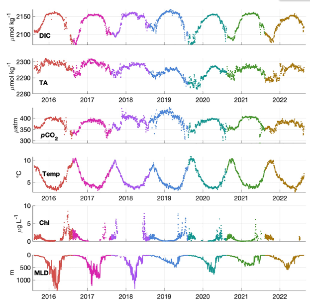
The time series results (Figure 3) showed that carbon system variables (dissolved inorganic carbon (DIC), total alkalinity (TA), and partial pressure of CO2 (pCO2)) co-vary through the annual cycle, with minimums in late summer at the end of the productive season and maximums in winter. The summer draw-down of pCO2 indicates that biophysical effects, rather than temperature, are the primary drivers of pCO2 variability. The influence of vertical mixing and primary productivity can be clearly seen in DIC and TA. In the subpolar North Atlantic, shoaling of the mixed layer in spring is generally associated with spring phytoplankton blooms, as indicated by increasing chlorophyll (Chl) concentration. Interestingly, it is found that highest integrated rates of DIC removal from the mixed layer via photosynthesis take place prior to mixed layer shoaling.
After a thorough analysis that included mixed layer budgets of DIC and TA, followed by assessment of gas exchange, physical transport, and the hydrologic cycle, the authors conclude that strong biological drawdown is the primary removal mechanism of inorganic carbon from the mixed layer. Furthermore, they point out the importance of interannual variability in both the drivers of and resulting magnitude of surface carbon cycling. This is primarily due to variability in net community production. Acknowledging the challenges taken on by OOI to maintain an array in the Irminger Sea, the authors note that “collecting observational data is both costly and challenging, however if only 1 year of data is collected or multiple years are averaged together, [carbon system dynamics] … will be misrepresented.”
This project shows the potential for OOI data, with appropriate processing and analysis, to provide unique insights into the ocean carbon system. It is notable that the authors made a substantial effort to calibrate and combine data from multiple instruments and moorings, and to take advantage of ancillary data (e.g. gliders, OOI CTD casts, and non-OOI CTD casts) in their processing. Enabling this type of analysis was a goal in the design of the multi-platform OOI Arrays and shipboard validation protocols.
[caption id="attachment_34983" align="alignnone" width="623"] Time series of dissolved inorganic carbon (DIC), total alkalinity (TA), partial pressure of CO2 (pCO2) temperature, chlorophyll-a (Chl), and mixed layer depth (MLD) in the Irminger Sea mixed layer from 2015-2022. Colors identify annual cycles. From Yoder et al., 2024.[/caption]
___________________
References:
- Fogaren, K. E., Palevsky, H. I. (2023) Bottle-calibrated dissolved oxygen profiles from yearly turn-around cruises for the Ocean Observations Initiative (OOI) Irminger Sea Array 2014 – 2022. Biological and Chemical Oceanography Data Management Office (BCO-DMO). Version Date 2023-07-19 doi:10.26008/1912/bco-dmo.904721.1
- Palevsky, H.I., S. Clayton and 23 co-authors, (2023).OOI Biogeochemical Sensor Data: Best Practices & User Guide Global Ocean Observing System, 1(1.1), 1–135. https://doi.org/10.25607/OBP-1865.2
- Palevsky, H. I., Fogaren, K. E., Nicholson, D. P., Yoder, M. (2023) Supplementary discrete sample measurements of dissolved oxygen, dissolved inorganic carbon, and total alkalinity from Ocean Observatories Initiative (OOI) cruises to the Irminger Sea Array 2018-2019. Biological and Chemical Oceanography Data Management Office (BCO-DMO). Version Date 2023-07-19 doi:10.26008/1912/bco-dmo.904722.1
- Yoder, M. F., Palevsky, H. I., & Fogaren, K. E. (2024). Net community production and inorganic carbon cycling in the central Irminger Sea. J. Geophys. Res., 129, e2024JC021027. https://doi.org/10.1029/2024JC021027
Summer Science Tours: CGSN Engages Young Environmentalists
The U.S National Science Foundation (NSF) OOI Coastal and Global Scale Nodes (CGSN) Team at WHOI has had a busy summer of talks and tours. With the help of Mashpee Wampanoag WHOI Tribal Liaison and Native Land Conservancy (NLC) founding board officer, Leslie Jonas, CGSN hosted two notable sets of visitors in July and August 2024. The NLC is an Indigenous-led land conservation nonprofit based on Cape Cod that seeks to preserve land for future generations.
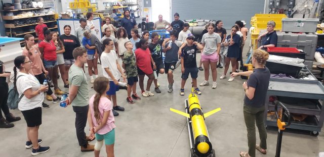
As a part of their Preserving Our Homelands (POH) summer science program, a group of students from the Mashpee Wampanoag tribe visited WHOI on 18 July. The POH program provides 6th, 7th, and 8th grade native students with hands-on science experiences in order to deepen their understanding of the environment from a western science perspective and its relationship to tribal culture, and traditional ecological knowledge. Their visit included a stop at the LOSOS facility, where CGSN team members talked about the scientific and technical aspects of the OOI program and provided an opportunity to see ocean observing technology up close. CGSN is grateful to WHOI engineer Ben Weiss and Sea Grant Marine Educator, Grace Simpkins, for organizing the visit and looks forward to ongoing interactions with the POH program.
Before the excitement from the POH tour had died down, a second group of visitors was hosted in early August. The group was made up of about 20 members of the Black, Indigenous, and People of Color (BIPOC) environmental science community. This included the NLC Executive Director, Diana Ruiz, and thirteen members of the Massachusetts Audubon Society and four NLC First Light Fellows. First Light is a paid summer fellowship program for rising Native American conservationists ages 18-25. With mentors from Mass Audubon, Fellows develop individual projects with topics in areas of ecological research, wetland restoration, water quality or land protection that build career skills and advance the NLC’s work. The fellowships combine indigenous culture, environmental sciences, and career development in order to open up career pathways. The four Indigenous Fellows who visited WHOI are studying at Brown, Yale, and Salish Kootenai College and got exposure to real-world instrumentation and engineering tools used to address pressing questions in ocean science research.
Read more about the NLC Fellows.
[caption id="attachment_34683" align="alignnone" width="640"] WHOI Senior Engineering Assistant Diana Wickman discusses the operation of an OOI ocean glider with Mashpee Wampanoag POH visitors. Photo credit J. Lund.[/caption]
[caption id="attachment_34684" align="alignnone" width="640"]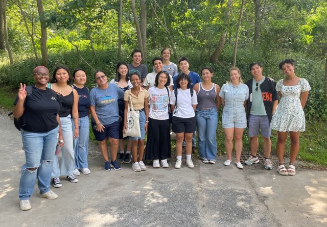 The August group included Native Land Conservancy First Light Fellows and members of the Massachusetts Audubon Society. Photo credit: L. Jonas.[/caption]
Read More
The August group included Native Land Conservancy First Light Fellows and members of the Massachusetts Audubon Society. Photo credit: L. Jonas.[/caption]
Read More Deep-Ocean Vertical Structure
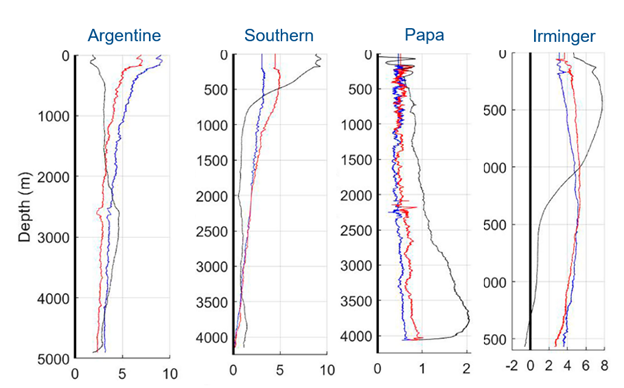
It is often assumed that, at frequencies below inertial, the vertical structure of horizontal velocity and vertical displacement can be reasonably described by a single dynamical mode, e.g. the lowest order flat-bottom baroclinic mode. This is appealing because it would mean that first-order predictions of deep-ocean velocity structure could be determined from knowledge of density and surface currents. However, there is a relative paucity of full ocean depth data to test this idea. A study by Toole et al. (2023) used full ocean depth data from five sites – four of which are Ocean Observatories Initiative (OOI) arrays (Station Papa, Irminger Sea, Argentine Basin and Southern Ocean) – to address the question “does subinertial ocean variability have a dominant vertical structure?”
Data analysis was challenging, because it involved working with gappy records as well as combining information from multiple instruments on different moorings. As noted by the authors, “no single OOI mooring sampled velocity, temperature and salinity over full depth.” Wire-following profiler data from Hybrid Profiler Moorings were combined with ADCP and fixed-depth CTD data from adjacent moorings. While the authors note that “depth-time contour plots of the velocity data from each OOI site clearly reveal the shortcomings of the datasets” they also recognized that despite the shortcomings, “these observations constitute some of the only full-depth observations of horizontal velocity and vertical displacement from the open ocean.”
It was possible to obtain 2-3 years (non-contiguous in some cases) of near-full ocean depth data from each site. Inertial and tidal variability was removed, and the data were filtered over 100 hr (~4 days). Empirical Orthogonal Function (EOF) decomposition was used to identify an orthogonal basis set that described horizontal velocity and vertical displacement. In addition, dynamical modes were determined for three cases: flat bottom, sloping bottom and rough bottom. Note that computing the dynamical modes requires the vertical density profile, which was taken as the mean over each deployment. Analysis was focused on the lowest modes, which accounted for the majority of the variance.
The results (Figure 32) showed that there is an EOF consistent with a dynamical mode at most sites. However, the appropriate dynamical mode is different for each site – no single dynamical accounted for a dominant fraction of variability across all sites. The authors note that differences in bathymetry, stratification and local forcing complicate the picture, with different dynamical processes dominating at different sites. Prior studies (not full ocean depth) that appear to show a “universal” vertical structure may be misleading
This project shows the potential for OOI data, with appropriate processing and analysis, to provide unique insights into ocean structure and dynamics. The researchers have made the combined vertical profile data available to the community on the Woods Hole Open Access Server. The dataset DOI (https://doi.org/10.26025/1912/66426) is also linked here: https://oceanobservatories.org/community-data-tools/community-datasets/.
[caption id="attachment_34586" align="alignnone" width="624"] Mode 1 EOFs for velocity (u, red; v blue; cm/s) and vertical displacement (black, decameters) for OOI arrays at (from left) Argentine Basin, Southern Ocean, Station Papa and Irminger Sea. Adapted from Toole et al., 2023.[/caption]
___________________
References:
Toole, J.M, R.C. Musgrave, E.C. Fine, J.M. Steinberg and R.A. Krishfield, 2023. On the Vertical Structure of Deep-Ocean Subinertial Variability, J. Phys. Oceanogr., 53(12), 2913-2932. DOI: 10.1175/JPO-D-23-0011.1.
Read MoreA Relationship Borne of OOI
OOI Engineer Jennifer Batryn had traveled to Punta Arenas, Chile in October 2016, to help mobilize for the third deployment and recovery cruise of the Global Argentine Basin Array. Punta Arenas is home to numerous street dogs, including a pack that slept in front of the hotel where the National Science Foundation Ocean Observatories Initiative (OOI) team was staying. On the way to begin work the first morning, Batryn stopped to pet several of the dogs and happily encouraged one to follow her to the warehouse facility where the team was working. He snuck through the port security entrance and joined Batryn and the team at the warehouse for the morning. When Batryn went into town for lunch, he followed and waited patiently outside of the restaurant. He then followed Batryn back to the warehouse for the afternoon and to the hotel at the end of the day. This pattern continued for the next week and a half while the team built and prepared the moorings.
[media-caption path="https://oceanobservatories.org/wp-content/uploads/2024/06/IMG_20161016_162823687-scaled.jpg" link="#"] OOI Instrument Lead Jennifer Batryn with her Punta Arenas Street dog, Teddy, outside the hotel in Chile. [/media-caption][media-caption path="https://oceanobservatories.org/wp-content/uploads/2024/06/IMG_20161011_113630857-scaled.jpg" link="#"]Teddy relaxing (and waiting for pets) outside the warehouse in the Punta Arenas port facility.[/media-caption]
When it came time to start loading the R/V Nathaniel B Palmer, Batryn realized that this dog had weaseled its way into her heart and decided she wasn’t leaving Chile without him. (Editor’s note: After looking into Teddy’s eyes, it is easy to understand how this happened!). “Teddy had the sweetest and most laid-back personality. He loved getting belly rubs and pats but also was content napping on a piece of foam in the warehouse, completely unfazed by the forklift trucks and other commotion going on. He was also amazingly dirty from living on the streets and my hands would instantly get a black film on them after petting him, but there was no way I could say no to him, “said Batryn. She chose the name Teddy since he was like a big teddy bear and started looking into the many logistics necessary to bring him back home with her.
Batryn only had several days to figure everything out before boarding the ship for three weeks. Since there were no pet stores nearby, she walked to a large grocery store and purchased a collar, leash, and a large bag of dog food. She then found a local vet clinic through a web search and got the name and phone number of a local dogsitter from the port agent. With that information in hand, Batryn enlisted the help of a friendly hotel employee to make the necessary phone calls to schedule an appointment since her Spanish was limited. She lucked out and was able to arrange a vet appointment the next day and scheduled a taxi to pick her and Teddy up from the port and take them across town.
The next day was Teddy’s first day wearing a collar and leash. It took some getting used to as he watched the other street dogs running down the busy street chasing cars without being able to join in. It would be a day of many more firsts. When it came time for the taxi to pick Batryn and Teddy up from the port entrance, Teddy, who was used to chasing cars and not riding in one, wanted no part of getting inside the vehicle. The port security guard saw the struggle and kindly offered to help lift the nearly 60 lb. dog into the back of the taxi. During the stressful ride across town, Batryn tried to comfort Teddy. When they arrived at the vet office, the front desk assistant saw Batryn’s dirty hands and exclaimed, “Ahh, mecánica!” assuming the black film on her hands was due to work as a mechanic, and not the result of petting a dirty street dog.
Batryn had previously read that Chile is free of dog rabies and that rabies vaccines were not required from that origin, but she decided to play it safe to help ensure smooth entry into the United States. She had Teddy receive all the basic shots necessary for travel, as well as a rabies shot and a certificate from the vet that Teddy was cleared for travel. Since it would be mid-November by the time they flew back to New England together, Batryn also got a signed notice that Teddy was acclimated to cold temperatures, having lived outside on the streets of Punta Arenas. This would increase the chances that the airlines would allow Teddy to travel if air temperatures happened to dip on their planned travel day. Teddy then had to endure a second cab ride to the dog sitters where he would live for the next several weeks while Batryn was at sea.
The logistics of bringing Teddy back home continued for Batryn during her three weeks at sea. In her down time between mooring operations, she used the limited ship Wi-Fi to call family and friends back home. She coordinated with her mother in California to purchase a dog kennel suitable for airline travel and asked a friend who was flying down to join her for hiking afterwards to take the giant kennel as a second piece of checked luggage. Batryn also enlisted the help of an Argentinian guest student onboard the Palmer to help call the dog sitter back in Punta Arenas to have her measure Teddy for properly sizing a kennel. The sitter also offered to give Teddy a much-needed bath before his travel to the US. The sitter later described this process to Batryn in a mix of Spanish and English as the dirtiest bath he’s ever given, with the water coming off Teddy looking “like coffee”.
Air travel is not permitted for the first four weeks after receiving a rabies vaccine, but Batryn’s time at sea combined with her week of hiking with her friend turned out to be perfect for the human-canine match. After a successful cruise and hike, Batryn reunited with her dog, but there was a small hitch. The dog kennel that her friend brought down was borderline too small for Teddy and had the potential to be rejected based on the airline guidelines. Not to be deterred, Batryn called upon the good graces of her dog sitter who traded the new kennel for an older, larger one that would allow Teddy to be more comfortable during his nearly 24-hour journey to Boston.
[media-caption path="https://oceanobservatories.org/wp-content/uploads/2024/06/DSC_3365-scaled.jpg" link="#"]Jennifer’s layover in Santiago was long enough to allow for picking up Teddy from the separate cargo area and a nice pit stop for him outside before the next big flight.[/media-caption]The big travel day went relatively smoothly. Due to the size of the new, larger kennel, Teddy had to fly with cargo on the first leg of the journey from Punta Arenas up to Santiago. That meant that Batryn had to exit the airport in Santiago to claim Teddy from a separate cargo area. Fortunately, a friendly cab driver outside the airport offered to walk with Batryn down the street to the cargo section. The next leg of the journey took Batryn and Teddy from Santiago, Chile, up to Miami, Florida. When claiming luggage to clear US customs, the large kennel again proved difficult as it was too large to fit on a standard luggage cart. Fortunately, a helpful airport employee helped load Teddy in his crate onto a larger airport cart and escorted them through customs. Much to Batryn’s surprise, they breezed through customs, despite bringing in a live animal from another country. The new team caught their final flight up to Boston and soon enough Batryn and Teddy were in Massachusetts on their way home to Cape Cod.
Once home, Teddy quickly settled into the idea of a more pampered life with comfortable beds, couches, regular meals, walks to the beach, and lots of attention. While he had to work through some initial separation anxiety, Teddy started coming into the LOSOS facility at Woods Hole Oceanographic Institution after just a couple days of being in the US. Ever since, Teddy has become a gentle fixture at LOSOS, getting pets from everyone who passes by, and spreading Chilean hospitality and good cheer every day.
Read More