
Bottom Boundary Layer O2 Fluxes During Winter on the Oregon Shelf
Adapted and condensed by OOI from Reimers et al., 2022, doi:/10.1029/2020JC016828.
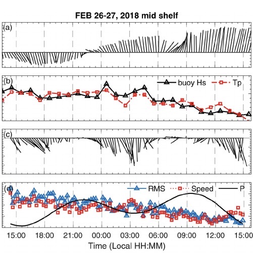
[caption id="attachment_21037" align="aligncenter" width="640"] Fig. 1 Time series of physical conditions during the February 26–27, 2018 deployment (EC D1) at the mid-shelf site. (a) Wind vectors (15-min averages) measured at the OOI Shelf Surface Mooring (CE02SHSM), (b) wave properties (hourly averages) measured at the OOI Shelf Surface Mooring, (c and d) other near-bottom ADV parameters (15-min averages). Both the winds and ADV velocities are portrayed in earth coordinates (eastward is to the right along the horizontal axis and northward is positive along the vertical axis). ADV, Acoustic Doppler Velocimeter; EC D, eddy covariance deployment[/caption]
The oceanic bottom boundary layer (BBL) is the portion of the water column close to the seafloor where water motions and properties are influenced significantly by the seabed. This study (Reimers & Fogaren, 2021) reported in the Journal of Geophysical Research examines conditions in the BBL in winter on the Oregon shelf. Dynamic rates of sediment oxygen consumption (explicitly oxygen fluxes) are derived from high-frequency, near-seafloor measurements made at water depths of 30 and 80 meters. The strong back-and-forth motions of waves, which in winter form sand ripples, pump oxygen into surface sediments, and contribute to the generation of turbulence in the BBL, were found to have primed the seabed for higher oxygen uptake rates than observed previously in summer.
Since oxygen is used primarily in biological reactions that also consume organic matter, the winter rates of oxygen utilization indicate that sources of organic matter are retained in, or introduced to, the BBL throughout the year. These findings counter former descriptions of this ecosystem as one where organic matter is largely transported off the shelf during winter. This new understanding highlights the importance of adding variable rates of local seafloor oxygen consumption and organic carbon retention, with circulation and stratification conditions, into model predictions of the seasonal cycle of oxygen.
Supporting observations, which give environmental context for the benthic eddy covariance (EC) oxygen flux measurements, include data from instruments contained in OOI’s Endurance Array Benthic Experiment Package and Shelf Surface Moorings. Specifically, velocity profile time-series are drawn from records of a 300-kHz Velocity Profiler (Teledyne RDI-Workhorse Monitor), near-seabed water properties from CTD (SBE 16plusV2) and oxygen (Aanderaa-Optode 4831) sensors, winds from the surface buoy’s bulk meteorological package, and surface-wave data products from a directional wave sensor (AXYS Technologies) (see e.g., Fig 1 above).
Reimers, C. E., & Fogaren, K. E. (2021). Bottom boundary layer oxygen fluxes during winter on the Oregon shelf. Journal of Geophysical Research: Oceans, 126, e2020JC016828. https://doi.org/10.1029/2020JC016828
Read More
Assimilative Model Assessment of Pioneer Array Data
Adapted and condensed by OOI from Levin et al., 2020, doi:/10.1016/j.ocemod.2020.101721.
[caption id="attachment_21009" align="alignnone" width="974"]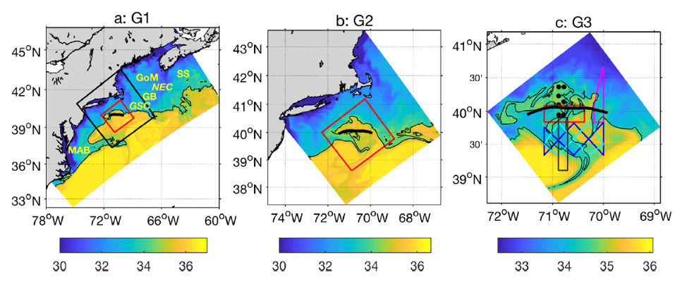 Fig. 1. Color contours of sea surface salinity from the model for three nested grids denoted a) G1, b) G2 (black square in (a)) and c) G3 (red square in (a), (b)). An indicator of frontal position (the 34.5 isohaline) is shown as a black contour. Cross-shelf exchange parameters are computed for an along-shelf section (thick black line). The Pioneer Array assets are shown in the G3 figure.[/caption]
Among the detailed analyses undertaken in this two-part study was quantification of the impact of observations on the reduction of RMS error for estimates of the volume transport across an along-front transect (Fig. 1). Temperature and salinity data from moorings and gliders were impactful for the larger grids (G1, G2). As the grid resolution was increased (G3), submesoscale motions were resolved and velocity data from the moorings became more important for reduction of error variance. An analysis of the sensitivity of shelf-slope exchange indices (e.g. volume transport) to removal of an observation, compared to the direct impact of the observation, showed that the majority of observed variables (e.g., SST, SSH, T, S, U, V) were “synergistic” – providing value to the assimilation through their connection with other variables as represented in the model dynamics. For the highest resolution estimates (G3 grid), the Pioneer Array observing assets were more impactful than other observations (e.g., remote sensing, NDBC and IOOS buoys) in reducing uncertainty, with velocity data being the major contributor. This is not a complete surprise, since the Pioneer Array was “tuned” to these scales. Still, it is gratifying to see that the impact on model fidelity is quantifiable.
The two-part study undertaken by Levin et al. provides a wealth of additional information about the performance of assimilative models as well as the utility of in-situ observations for modeling and prediction. As the authors state, they have “just begun to scratch the surface” of approaches that can be applied to the assessment of model performance as well as the management of observing systems.
Levin J., H.G. Arango, B. Laughlin, E. Hunter, J. Wilkin, and A.M. Moore, 2020. Observation impacts on the Mid-Atlantic Bight front and cross-shelf transport in 4D-Var ocean state estimates: Part I – Multiplatform analysis,Ocean Modeling, 156, 101721, 1-17, doi 10.1016/j.ocemod.2020.101721.
Read More
PI Cabled Instrument Provides Real-Time Sonar Measurements of Hydrothermal Plume Emissions
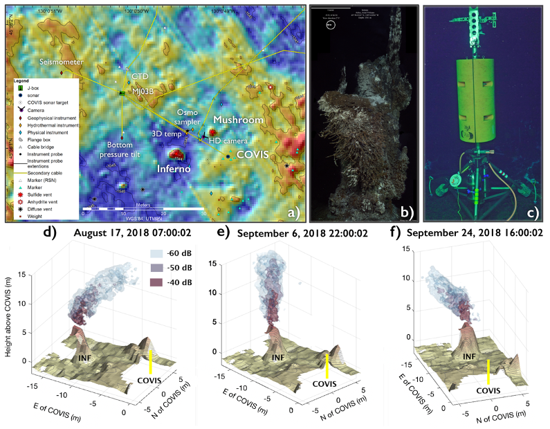
Adapted and condensed by OOI from Xu et al., 2022, doi:/10.1029/2020EA001269.
[media-caption path="https://oceanobservatories.org/wp-content/uploads/2021/02/RCA-FOR-SCIENCE-HIGHLIGHTS.png" link="#"]Figure 26. a) Location of the COVIS sonar and RCA infrastructure in the ASHES Hydrothermal Field. Also shown are locations of the active ~ 4 m tall hydrothermal edifices ‘Mushroom’ and ‘Inferno’. c) The COVIS sonar in 2019 (Credit: Rutgers/UW/NSF-OOI/WHOI). The tower is 4.2 m tall and hosts a modified Reson 7125 SeaBat multibeam sonar mounted on a tri-axial rotator. The system was built by the UW Applied Physics Laboratory. d) Selected time-series images from COVIS showing bending of the plume eastward, e) a nearly vertical plume, and f) southward bending of the plume (after Fig. 7 Xu et al., 2020).[/media-caption]The Cabled Observatory Vent Imaging Sonar (COVIS) was installed on the OOI RCA in the ASHES hydrothermal field (Fig. 26 a-c) at the summit of Axial Seamount in 2018, resulting in the first long-term, quantitative monitoring of plume emissions (Xu et al., 2020). The sonar provides 3-dimensional backscatter images of buoyant plumes above the actively venting ‘Inferno’ and ‘Mushroom’ edifices, and two-dimensional maps of diffuse flow at temporal frequencies of 15 and 2 minutes, respectively. Sonar data coupled with in-situ thermal measurements document significant changes in plume variations (Fig. 26 d-f) and modeling results indicate a heat flux of 10 MW for the Inferno plume (Xu et al., 2020). COVIS will provide key data to the community investigating the impacts of eruptions on hydrothermal flow at this highly active volcano.
[1] Xu, G., Bemis, K., Jackson, D., and Ivakin, A., (2020) Acoustic and in-situ observations of deep seafloor hydrothermal discharge: OOI Cabled Array ASHES vent field case study. Earth and Space Science. Note: This project was funded by the National Science Foundation through an award to PI Dr. K. Bemis, Rutgers University – “Collaborative Research: Heat flow mapping and quantification at ASHES hydrothermal vent field using an observatory imaging sonar (#1736702). COVIS data are available through oceanobservatories.org.
Read MoreEndurance Oregon Shelf Data Provides Insights into Bottom Boundary Layer Oxygen Fluxes
Adapted and condensed by OOI from Reimers et al., 2021, doi:/10.1029/2020JC016828
In February 2021 JGR Oceans article, Clare E. Reimers (Oregon State University) and Kristen Fogaren (Boston College) used data from the Endurance Array Oregon Shelf to advance understanding of how the benthic boundary layer on the Oregon Shelf in winter depends on surface-wave mixing and interactions with the seafloor.
The oceanic bottom boundary layer (BBL) is the portion of the water column close to the seafloor where water motions and properties are influenced significantly by the seabed. This study examines conditions in the BBL in winter on the Oregon shelf. Dynamic rates of sediment oxygen consumption (explicitly oxygen fluxes) are derived from high-frequency, near-seafloor measurements made at water depths of 30 and 80 m. The strong back-and-forth motions of waves, which in winter form sand ripples, pump oxygen into surface sediments, and contribute to the generation of turbulence in the BBL, were found to have primed the seabed for higher oxygen uptake rates than observed previously, in summer. Since oxygen is used primarily in biological reactions that also consume organic matter, the winter rates of oxygen utilization indicate that sources of organic matter are retained in, or introduced to, the BBL throughout the year. These findings counter former descriptions of this ecosystem as one where organic matter is largely transported off the shelf during winter. This new understanding highlights the importance of adding variable rates of local seafloor oxygen consumption and organic carbon retention, with circulation and stratification conditions, into model predictions of the seasonal cycle of oxygen.
The rest of the article can be accessed here.
Read More
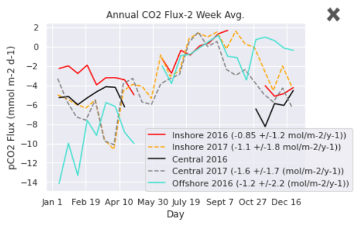
Pioneer Data Show the Continental Shelf Acts as a Carbon Sink
Excerpted from the OOI Quarterly Report, 2022.
[media-caption path="https://oceanobservatories.org/wp-content/uploads/2021/02/Pioneer-for-Science-Highlights.png" link="#"]Figure 23. Weekly average air-sea CO2 flux estimated for the Pioneer Array Inshore, Central and Offshore moorings during 2016 and 2017. A negative flux is from the atmosphere to the ocean. From Thorson and Eveleth (2020).[/media-caption]In the summer of 2020 the Rutgers University Ocean Data Labs project worked with the Rutgers Research Internships in Ocean Science to support ten undergraduate students in a virtual Research Experiences for Undergraduates program. Two weeks of research methods training and Python coding instruction was followed by six weeks of independent study with a research mentor.
Dr. Rachel Eveleth (Oberlin College) was one of those mentors. Already using some of the Data Labs materials in her undergraduate oceanography course, she saw an opportunity to leverage the extensive OOI data holdings to engage students in cutting edge research on a limited budget during a time when her own field work was curtailed due to the COVID-19 pandemic. Dr. Eveleth advised Alison Thorson from Sarah Lawrence College (NY) and Brianna Velasco form Humboldt State University (CA) on the study of air-sea fluxes of CO2 on the US east and west coast, respectively.
Preliminary results were presented at the 2020 Fall AGU meeting. A poster authored by Thorson and Eveleth (ED037-0035) evaluated pCO2 data from the three Pioneer Array Surface Moorings during 2016 and 2017. They showed that the annual mean CO2 flux across all three sites for the two years was negative, meaning that the continental shelf acts as a sink of atmospheric carbon. The annual average flux was -0.85 to -1.6 mol C/(m2 yr), but the flux varied significantly between mooring sites and between years (Figure 23). Investigation of short-term variability in pCO2 concentration concurrent with satellite imagery of SST and Chlorophyll was consistent with temperature-driven, but biologically damped, changes.
[media-caption path="https://oceanobservatories.org/wp-content/uploads/2021/02/Pioneer-for-Science-Highlights.png" link="#"]Figure 24. Hourly (dots) and monthly (lines) average air and water CO2 concentration observed at the Endurance Array Washington Offshore mooring during 2016 and 2017. From Velasco et al. (2020).[/media-caption]A poster by Velasco, Eveleth and Thorson (ED004-0045) analyzed pCO2 data from the Endurance Array offshore mooring. Three years of nearly continuous data were available during 2016-2018. The seasonal cycle showed that the pCO2 concentration in water was relatively stable and near equilibrium with the air in winter, decreasing in late spring and summer (Figure 24). Short-term minima in summer were as low as 150 uatm. Like the east coast, the mean air-sea CO2 flux was consistently negative, meaning the coastal ocean acts as a carbon sink. The annual means at the Washington Offshore mooring for 2016, 2017 were -1.9 and -2.1 mol C/(m2 yr), respectively. The seasonal cycle appears to be strongly driven by non-thermal factors (on short time scales), presumably upwelling events and algal blooms.
These studies, although preliminary, are among the first to use multi-year records of in-situ CO2 flux from the OOI coastal arrays, and to our knowledge the first to compare such records between the east and west coast. Dr. Eveleth’s team intends to use the rich, complementary data set available from the OOI coastal arrays to investigate the mechanisms controlling variability and role of biological vs physical drivers.
Read More
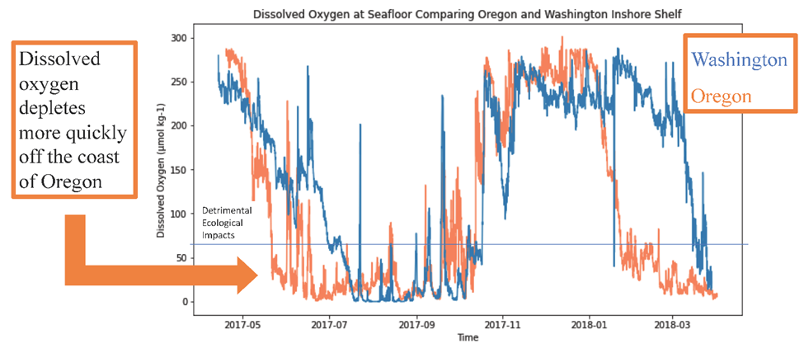
Low Dissolved Oxygen off Washington and Oregon Coast Impacted by Upwelling in 2017
In the summer of 2020, the Rutgers University Ocean Data Labs project worked with the Rutgers Research Internships in Ocean Science to support ten undergraduate students in a virtual Research Experiences for Undergraduates program. Rutgers led two weeks of research methods training and Python coding instruction. This was followed by six weeks of independent study with one of 13 research mentors.
Dr. Tom Connolly (Moss Landing Marine Labs, San Jose State University) advised Andrea Selkow from Austin College, Texas on her study of dissolved oxygen (DO) off the Washington and Oregon coasts using the OOI Endurance Array.
Selkow evaluated DO data from Endurance Array Surface Moorings during 2017 and 2018. She presented this work as a poster at the conclusion of her summer REU. Selkow focused on the question: Are there similarities in the dissolved oxygen concentrations off the coast of Oregon and Washington during a known low oxygen event? She also considered why there might exist differences based on the spatial variability of wind stress forcing, i.e., do the strong Oregon winds cause dissolved oxygen concentrations to be lower at the Oregon mooring compared to the Washington moorings. Finally, she reviewed the data and tried to answer whether the oxygen data were accurate or affected by biofouling.
She used datasets from the OR and WA Inshore Shelf Mooring time-series and WA Shelf Mooring time-series from Endurance Array. Her focus was on the seafloor data because that is where the lowest oxygen concentrations were expected to be observed.
Selkow focused her attention on low DO observed in the summer of 2017. While Barth et al. (2018) presented a report on these data for one event in July 2017, she expanded the analysis to include the Washington shelf and inshore moorings. She plotted time series data and used cruise data to validate these time series. While overall seasonal trends in DO were similar, she found dissolved oxygen is routinely more quickly depleted off the coast of Oregon than Washington during a low oxygen event (Figure 25). She also looked at the cross-shelf variability in DO time series and found dissolved oxygen is more quickly depleted at the shelf mooring than at the inshore shelf mooring. Upwelling is known to drive the low oxygen events and she inferred that the weaker southward winds over the Washington shelf may be why DO decreases at a slower rate off Washington than Oregon.
References
Barth, J.A., J.P. Fram, E.P. Dever, C.M. Risien, C.E. Wingard, R.W. Collier, and T.D. Kearney. 2018. Warm blobs, low-oxygen events, and an eclipse: The Ocean Observatories Initiative Endurance Array captures them all. Oceanography 31(1):90–97,
Selkow, A. and T. Connelly. Low Dissolved Oxygen off Washington and Oregon Coast Impacted by Upwelling in 2017, Accessed 13 Jan 2021.
Read MoreBuoy Wave Height Measurements Improve SAR Estimates
Excerpted from the OOI Quarterly Report, 2022.
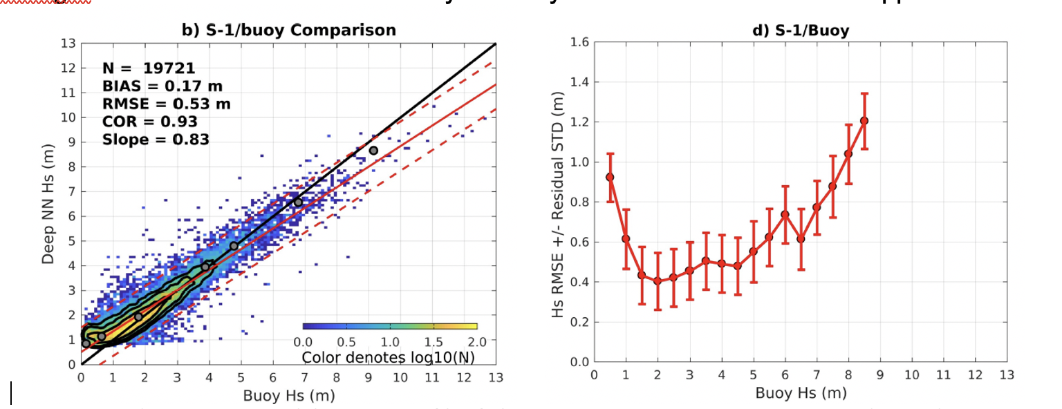
Synthetic Aperture Radar (SAR) sensors on satellites measure backscatter from the ocean surface and can be used to estimate wave height at very high spatial resolution (~10 m) relative to satellite altimetry. Two Sentinel-1 satellites of the European Space Agency (ESA) collected SAR measurements of the ocean surface from 2015-2018, together covering the entire globe every six days. Data-driven approaches to predicting significant wave height (Hs) from SAR have either used relatively limited in-situ data sets or used a wave model (e.g. WaveWatch-3) as the “training” data for a deep learning approach. Quach et al.(2020) improve on previous approaches to estimation of Hs from SAR by creating a comprehensive in-situ observational record. They compiled data from the US National Data Buoy Center and Coastal Data Information Program, Canadian Marine Environmental Data Services, the international OceanSITES project, and the OOI. Surface wave data sets from the OOI Irminger Sea, Argentine Basin and Southern Ocean surface buoys were used. The authors note the importance of the Southern Ocean Array, where “many of the largest wave heights are recorded… [from] an under sampled region of the ocean.”
The comprehensive in-situ data set is split into separate training and validation segments. When SAR Hs from training data are compared to altimeter Hs from the validation segment, the deep learning algorithm shows root-mean-square (RMS) error of 0.3 m, a 50% improvement relative to prior approaches. Comparison with the buoy validation segment (Fig. 18) shows RMS error of 0.5 m. The authors attribute the increased error to the larger number of extreme sea states in the observations and the relative paucity of extremes in the training data.
Observational sea state information is critical for understanding surface wave phenomena (generation, propagation and decay), predicting wave amplitudes, and estimating extreme sea states. Thus, the improvement in RMS error using the deep learning technique notable. The availability of in-situ data from extreme environments such as those sampled by the OOI Irminger Sea and Southern Ocean Arrays are key to validation of these new approaches.
.
Read MoreUnderstanding Factors Controlling Seismic Activity Along the Cascadia Margin
Excerpted from the OOI Quarterly Report, 2022.
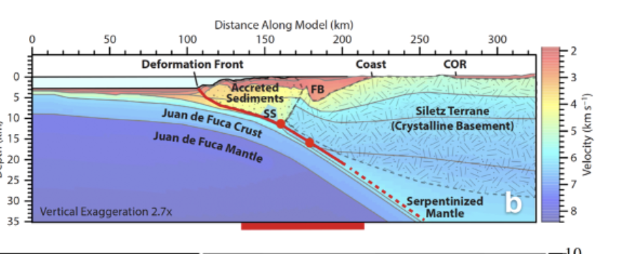
The Cascadia Subduction Zone extends from northern California to British Columbia. It has experienced magnitude 9 megathrust events with a reoccurrence rate of every ~500 years over the past 10,000 years [5] and large earthquakes at intervals of ~ 200-1200 years [6]. The last Cascadia megathrust rupture occurred on January 26, 1700 [5]. When the next event occurs, it is estimated that financial losses would be ~ $60 billion USD with substantial loss of life. Hence, there is significant research focused on understanding seismic processes along this ~ 1100 km subduction zone, the generation of slow earthquakes, and causes of variation in seismicity along strike.
[media-caption path="/wp-content/uploads/2020/10/RCA-science-highlight-pic.png" link="#"]Figure 20. Earthquake generating processes in the central portion of the Cascadia Margin. a) Location of ≥4 magnitude earthquakes (red dots) 1989-August 2017 from the Advanced National Seismic System Comprehensive Earthquake catalog. The short dashed line is the 450°C contour, and short-long dashed line is the updip limit of tremor from 2005-2011 [after 1]. b) Interpreted cross section through the Cascadia Subduction Zone crossing the location of the Regional Cabled Array (RCA) margin sites. Red dots are projected positions of two 4.7-4.8 magnitude earthquakes in 2004 [1]. Basement rocks of the upper plate – the Siletz Terrane – comprise accreted anomalously thick mafic oceanic crust [1-3]. SS indicates the position of a subducted seamount west of the Siletz terrane [1]. c) Detected seismicity (blue dots – 222 earthquakes) approximately centered on the location of RCA ocean bottom seismometers on the Juan de Fuca Plate at Slope Base and on the margin at Southern Hydrate Ridge (purple triangles) [4]. Dot size is proportional to magnitude. A southern cluster centered at depths of ~ 5-10 km, is associated with the location of the subducted seamount, while the northern cluster may be associated with possibly accreted seamount [4].)[/media-caption]Understanding the factors that control seismic events was/is a major driver in the siting of OOI-RCA core geophysical instrumentation on the southern line of the Regional Cabled Array: the RCA is one of the few places in the world where seismic-focused instrumentation occurs on both the down-going tectonic plate and on the overlying margin. The offshore network is especially valuable in determining earthquake source depths that inform on interpolate dynamics [1]. The central section of the Cascadia Margin is the only area that experiences repeat, measurable shallow crustal earthquakes [1-3]. RCA data flowing from the seismic network at Slope Base and Southern Hydrate Ridge, and from the Cascadia Initiative are providing new insights into factors controlling seismicity along this portion of the margin [1,4] (note because the RCA broadband seismometers are buried, they have lower noise levels at higher frequencies than the Cascadia Initiative instruments [1]).
Most recently, Morton et al., [4] examined data from the Cascadia Initiative [7] and the RCA. Shallow earthquakes are focused in the area of a subducted seamount [1-3] and another cluster to the north (Fig. 1b and c). Based on earthquake locations, they suggest that subduction of the seamount produces stress heterogeneities, faulting, fracturing of the overriding Siletz terrane (old oceanic crust) (Fig 1b), and fluid movement promoting seismic swarms. Because this area is the most seismically active area along the Cascadia margin, it is an optimal area to examine the impacts of local earthquakes on, for example, gas hydrate deposits and fluid expulsion.
[1] Tréhu, A.M., Wilcock, W.S.D., Hilmo, R., Bodin, P., Connolly, J., Roland, E.C., and Braunmiller, R., (2018) The role of the Ocean Observatories Initiative in Monitoring the offshore earthquake activity of the Cascadia Subduction Zone. Oceanography, 31, 104-113.
[2] Tréhu, A.M., Blakely, R.J., and Williams, M., (2012) Subducted seamounts and recent earthquakes beneath the central Cascadia Forearc. Geology, 40, 103-106.
[3] Tréhu, A.M., Braunmiller, J., and Davis, E., (2015) Seismicity of the Central Cascadia Continental Margin near 44.5° N: a decadal view. Seismological Research Letters, 86, 819-829.
[4] Morton, Bilek, S.L., and Rowe, C.A. (2018) Newly detected earthquakes in the Cascadia subduction zone linked to seamount subduction and deformed upper plate. Geology, 46, 943-946.
[5] Satake, K.Shimazaki, K., Tsuji, Y., and Ueda, K., (1996) Time and size of a giant earthquake in Cascadia inferred from Japanese tsunami records of January 1700. Nature, 379, 246-249.
[6] Goldfinger, C., Nelson, C.H., Eriksson, E., et al., (2012) Turbidite event history: Methods and implications for Holocene paleoseismicity of the Cascadia Subduction Zone. US Geological Survey Professional Paper (1661-F), 184 pp.
[7] Toomey, D.R., Allen, R.M., Barclay, A.H., Bell, S.W., Bromirski, P.D. et al., (2014) The Cascadia Initiative: A sea change in seismological studies of subduction zones. Oceanography, 27, 138-150.
Read More
Delineating Biochemical Processes in the Northern California Upwelling System
Excerpted from the OOI Quarterly Report, 2022.
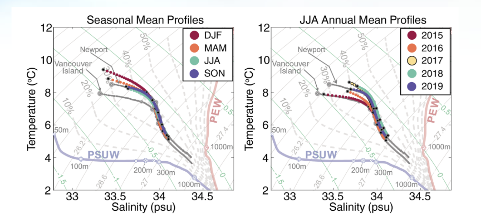
[media-caption path="/wp-content/uploads/2020/10/Endurance-Array-Science-Highlight.png" link="#"]Figure 19: Regional T/S variability at the Washington offshore profiling mooring. The end member Pacific Subarctic Upper Water (PSUW) and Pacific Equatorial Water (PEW) masses are indicated on each plot at the left and right respectively. T/S at the mooring is a mixture of PSUW and PEW. The left plot shows the seasonal variability. The right plot shows interannual variability in summer. Interannual variability from 100-250m exceeds seasonal variability. In 2015, T/S at the mooring is closer in character to climatological averages at Vancouver Island, BC while in 2018, T/S at the mooring is similar to that south of Newport, OR. Figure from Risien et al. adapted from Thomson and Krassovski (2010).[/media-caption]
Risien et al. (2020) presented over five years of observations from the OOI Washington offshore profiling mooring. First deployed in 2014, the Washington offshore profiler mooring is on the continental slope about 65 km west of Westport, WA. Its wire Following Profiler samples the water column from 30 m depth down to 500 m, ascending and descending three to four times per day. Traveling at approximately 25 cm/s, the profiler carries physical (temperature, salinity, pressure, and velocity) and biochemical (photosynthetically active radiation, chlorophyll, colored dissolved organic matter fluorescence, optical backscatter, and dissolved oxygen) sensors. The data presented included more than 12,000 profiles. These data were processed using a newly developed Matlab toolbox.
The observations resolve biochemical processes such as carbon export and dissolved oxygen variability in the deep source waters of the Northern California Upwelling System. Within the Northern California Current System, over the slope there is a large-scale north-south variation in temperature and salinity (T/S). Regional T/S variability can be understood as a mixing between warmer, more saline Pacific Equatorial Water (PEW) to the south, and fresher, colder Pacific Subarctic Upper Water (PSUW) to the north. Preliminary results show significant interannual variability of T/S water properties between 100-250 meters. In summer, interannual T/S variability is larger than the mean seasonal cycle (see Fig 19). While summer T/S variability is greatest on the interannual scale, T/S does covary on a seasonal scale with dissolved Oxygen (DO), spiciness and Particulate Organic Carbon (POC). In particular, warmer, more saline water is associated with lower DO in fall and winter.
Risien, C.M., R.A. Desiderio, L.W. Juranek, and J.P. Fram (2020), Sustained, High-Resolution Profiler Observations from the Washington Continental Slope , Abstract [IS43A-05] presented at Ocean Sciences Meeting 2020, San Diego, CA, 17-21 Feb.
Thomson, R. E., and Krassovski, M. V. (2010), Poleward reach of the California Undercurrent extension, J. Geophys. Res., 115, C09027, doi:10.1029/2010JC006280.
Read More
Discovery of the Roots of the Axial Seamount
Excerpted from the OOI Quarterly Report, 2020.
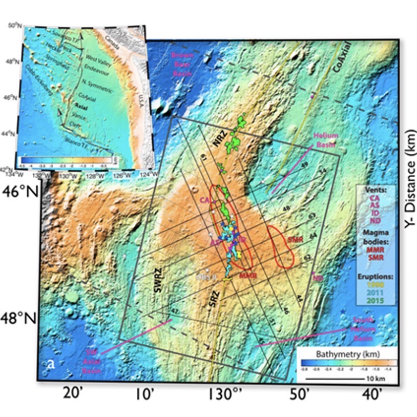
[media-caption type="image" class="external" path="https://oceanobservatories.org/wp-content/uploads/2020/09/Screen-Shot-2020-09-17-at-1.21.46-PM.png" alt="Axial Seamount Roots" link="#"]. Figure 14: a) Location of 1998, 2011, and 2015 lava flows at the summit of Axial Seamount, two magma chambers (re outlines MMR & SMR) and seismic lines (after [1]). b) Map view and perspective view of the MMR magma reservoir, seismicity and fault mechanisms from 10/2014 to 9/2015 (after [1]).[/media-caption]Two- and 3D-imaging of Axial Seamount, coupled with real-time monitoring of seismicity and seafloor deformation, is providing unprecedented insights into submarine volcanism, the nature of melt transport, and caldera dynamics (Figure 14) [1-15]. Recently acquired 3D imaging of the volcano [2] and analyses of 1999 and 2002 multichannel seismic data [4-7] have led to the remarkable discovery of a root zone 6 km beneath the volcano [2,5]. Carbotte et al., [5] describe a 3-to-5 km wide conduit that is interpreted to be comprised of numerous quasi-horizontal melt lenses spaced 400-500 m apart. The conduit is located beneath a 14-km-long magma reservoir (MMR) that spans the caldera of Axial Seamount and a secondary, smaller magma chamber (SMR) located beneath the eastern flank of the volcano [1,3]. This smaller reservoir presumably Dymond hydrothermal field hosting up to 60 m-tall actively venting chimneys, which was discovered on a 2011 RCA cruise. Seismicity prior to, during and subsequent to the 2015 eruption delineates outward dipping normal faults in the southern half of the caldera that extend from near the seafloor to 3-3.25 km depth [3,8-9]. In contrast, a conjugate set of inward dipping faults in the northern portion of the caldera extend to depths of ~ 2.25 km. The outward dipping ring faults were active during inflation and syn-eruptive deformation [[3,8-9]. Source fissures for the 1998, 2011, and 2015 eruptions are located within ± 1 km of where the MMR roof is shallowest (<1.6 km beneath the seafloor) and skewed toward the eastern caldera wall [3]. In concert, these studies are changing long-held views of magma chamber geometry and the deep-rooted feeder systems in mid-ocean ridge environments [2,5].
[1] Arnulf, A. F., Harding, A. J., Kent, G. M., Carbotte, S. M., Canales, J. P., and Nedimovic, M. R. (2014) Anatomy of an active submarine volcano. Geology, 42(8), 655–658. https://doi.org/10.1130/G35629.1.
[2] Arnulf, A.F., Harding, A.J., Saustrup, S., Kell, A.M., Kent, G.M., Carbott, S.M., Canales, J.P., Nedimovic, M.R., Bellucci M., Brandt, S., Cap, A., Eischen, T.E., Goulin, M., Griffiths, M., Lee, M., Lucas, V., Mitchell, S.J., and Oller, B. (2019) Imaging the internal workings of Axial Seamount on the Juan de Fuca Ridge. American Geophysical Union, Fall Meeting 2019, OS51B-1483.
[3] Arnulf, A.F., Harding, A.J., Kent, G.M., and Wilcock, W.S.D. (2018) Structure, seismicity and accretionary processes at the hot-spot influenced Axial Seamount on the Juan de Fuca Ridge. Journal of Geophysical Research, 10.1029/2017JB015131.
[4] Carbotte, S. M., Nedimovic, M. R., Canales, J. P., Kent, G. M., Harding, A. J., and Marjanovic, M. (2008) Variable crustal structure along the Juan de Fuca Ridge: Influence of on-axis hot spots and absolute plate motions. Geochemistry, Geophysics, Geosystems, 9, Q08001. doi.org/10.1029/2007GC001922.
[5] Carbotte, S.M., Arnulf, A.F., Spiegelman, M.W., Harding, A.J., Kent, G.M., Canales, J.P., and Nedimovic, M.R. (2019) Seismic images of a deep melt-mush feeder conduit beneath Axial Volcano. American Geophysical Union, Fall Meeting 2019, OS51B-1484.
[6] West, M., Menke, W., and Tolstoy, M. (2003) Focused magma supply at the intersection of the Cobb hotspot and the Juan de Fuca ridge. Geophysical Research Letters, 30(14), 1724. https://doi.org/10.1029/2003GL017104.
[7] West, M., Menke, W., Tolstoy, M., Webb, S., and Sohn, R. (2001). Magma storage beneath Axial volcano on the Juan de Fuca mid-ocean ridge. Nature, 413(6858), 833–836. doi.org/10.1038/35101581.
[8] Wilcock, W.S.D., Tolstoy, M., Waldhauser, F., Garcia, C., Tan, Y.J., Bohnenstiehl, D.R., Caplan-Auerbach, J., Dziak, R., Arnulf, A.F., and Mann, M.E. (2016) Seismic constraints on caldera dynamics from the 2015 Axial Seamount eruption. Science, 354, 1395-399; https://doi.org/10.1126 /science.aah5563.
[9] Wilcock, W.S.D., Dziak, R.P., Tolstoy, M., Chadwick, W.W., Jr., Nooner, S.L., Bohnenstiehl, D.R., Caplan-Auerbach, J., Waldhauser, F., Arnulf, A.F., Baillard, C., Lau, T., Haxel, J.H., Tan, Y.J, Garcia, C., Levy, S., and Mann, M.E. (2018) The recent volcanic history of Axial Seamount: Geophysical insights into past eruption dynamics with an eye toward enhanced observations of future eruptions. Oceanography, 31,(1), 114-123.
[10] Chadwick, W.W., Jr., Nooner, S.L., and Lau, T.K.A. (2019) Forecasting the next eruption at Axial Seamount based on an inflation-predictable pattern of deformation. American Geophysical Union, Fall Meeting 2019, OS51B-1489.
[11] Chadwick, W.W., Jr., Paduan, J.B., Clague, D.A., Dreyer, B.M., Merle, S.G. Bobbitt, A.M. Bobbitt, Caress, D.W. Caress, Philip, B.T., Kelley, D.S., and Nooner, S. (2016) Voluminous eruption from a zoned magma body after an increase in supply rate at Axial Seamount. Geophysical Research Letters, 43, 12,063-12,070; https://doi. org/10.1002/2016GL071327.
[12] Nooner, S.L., and Chadwick, W.W. Jr. (2016) Inflation- predictable behavior and co-eruption deformation at Axial Seamount. Science, 354, 1399-1403; https://doi.org/10.1126/ science.aah4666.
[13] Nooner, S.L., and Chadwick, W.W. Jr. (2016) Inflation- predictable behavior and co-eruption deformation at Axial Seamount. Science, 354, 1399-1403; https://doi.org/10.1126/ science.aah4666.
[14] Hefner, W.L., Nooner, S.L., Chadwick, W.W., Jr., and Bohnenstiehl, D.R. (2020) Magmatic deformation models including caldera-ring faulting for the 2015 eruption of Axial Seamount. Journal of Geophysical Research, https://doi:10.1029/2020JB019356.
[15] Levy, S., Bohnenstiehl, D.R., Sprinkle, R., Boettcher, M.S., Wilcock, W.S.D., Tolstoy, M., and Waldhouser, F. (2018) Mechanics of fault reactivation before, during, and after the 2015 eruption of Axial Seamount. Geology, 46(5), 447-450; https://doi.org/10.1130/G39978.1.
Read More